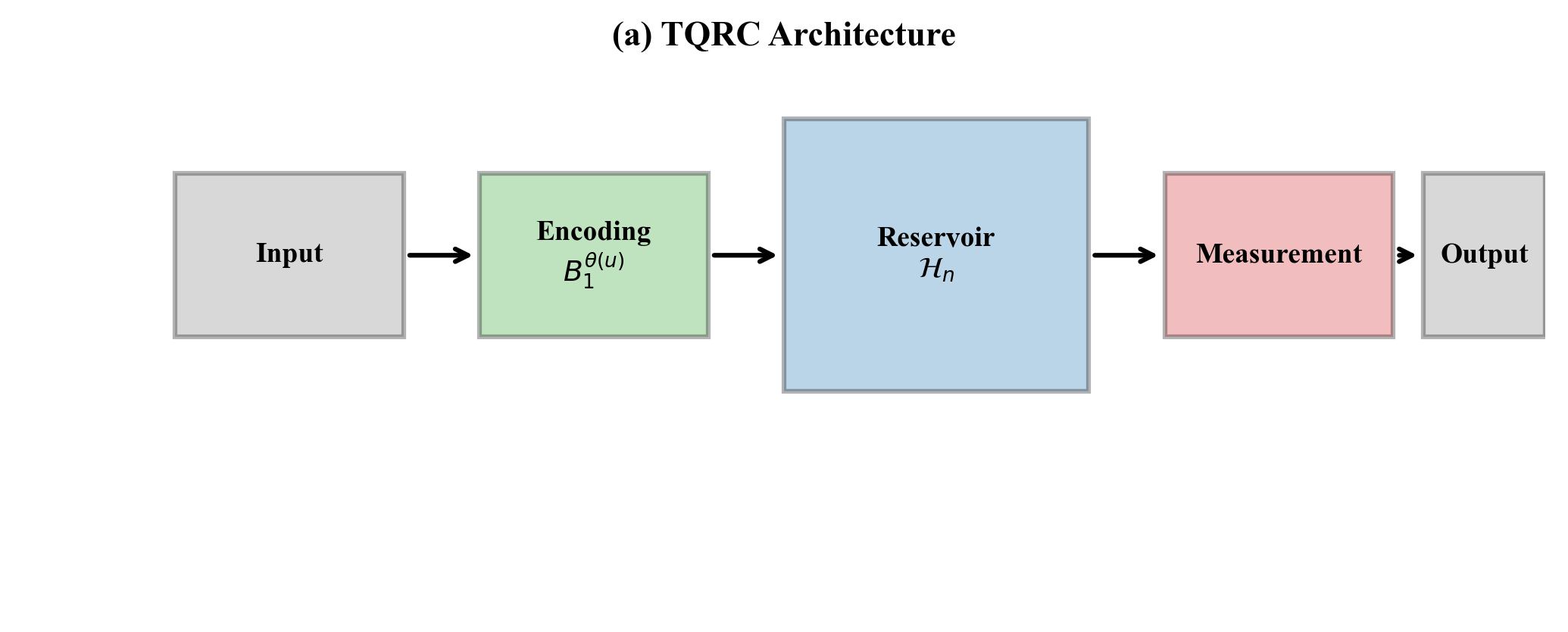
The Fundamental Tension in Topological Quantum Reservoir Computing

Topological quantum computing promises fault-tolerant quantum operations protected by the geometry of space itself. Reservoir computing promises powerful machine learning without complex training. What happens when you combine them?

Nothing good, as it turns out. In this paper, we prove a fundamental no-go theorem: the properties that make topological systems attractive for quantum computing are exactly what makes them impossible to use as reservoirs.

This is not an engineering problem to be solved with better technology. It is a mathematical incompatibility rooted in the foundations of quantum mechanics.

Version 2 Update (January 2026): This article reflects the revised paper with 30-trial statistical validation, bootstrap 95% confidence intervals, new quantum state evolution visualizations (Figure 9), NARMA-10 benchmark results, and updated literature through 2025 including Google and Quantinuum Fibonacci anyon demonstrations.

What Are Anyons?

To understand our result, we first need to understand the exotic particles called anyons.

In three dimensions, particles come in two types: fermions and bosons. Fermions (like electrons) obey the Pauli exclusion principle. Two fermions cannot occupy the same quantum state. Bosons (like photons) are the opposite. They prefer to bunch together in the same state.

In two dimensions, something remarkable happens. The topology of space allows for particles that are neither fermions nor bosons. These are anyons. When you exchange two anyons by moving them around each other, the quantum state picks up a phase that can be any value between 0 and 2π.

Even more exotic are non-abelian anyons. When you exchange non-abelian anyons, the quantum state does not just pick up a phase. It undergoes a matrix transformation. The order in which you exchange anyons matters. Different exchange sequences produce different quantum states.

This is profoundly different from ordinary particles. Exchanging electrons A and B, then B and C, gives the same result as exchanging B and C first, then A and B. For non-abelian anyons, the order matters.

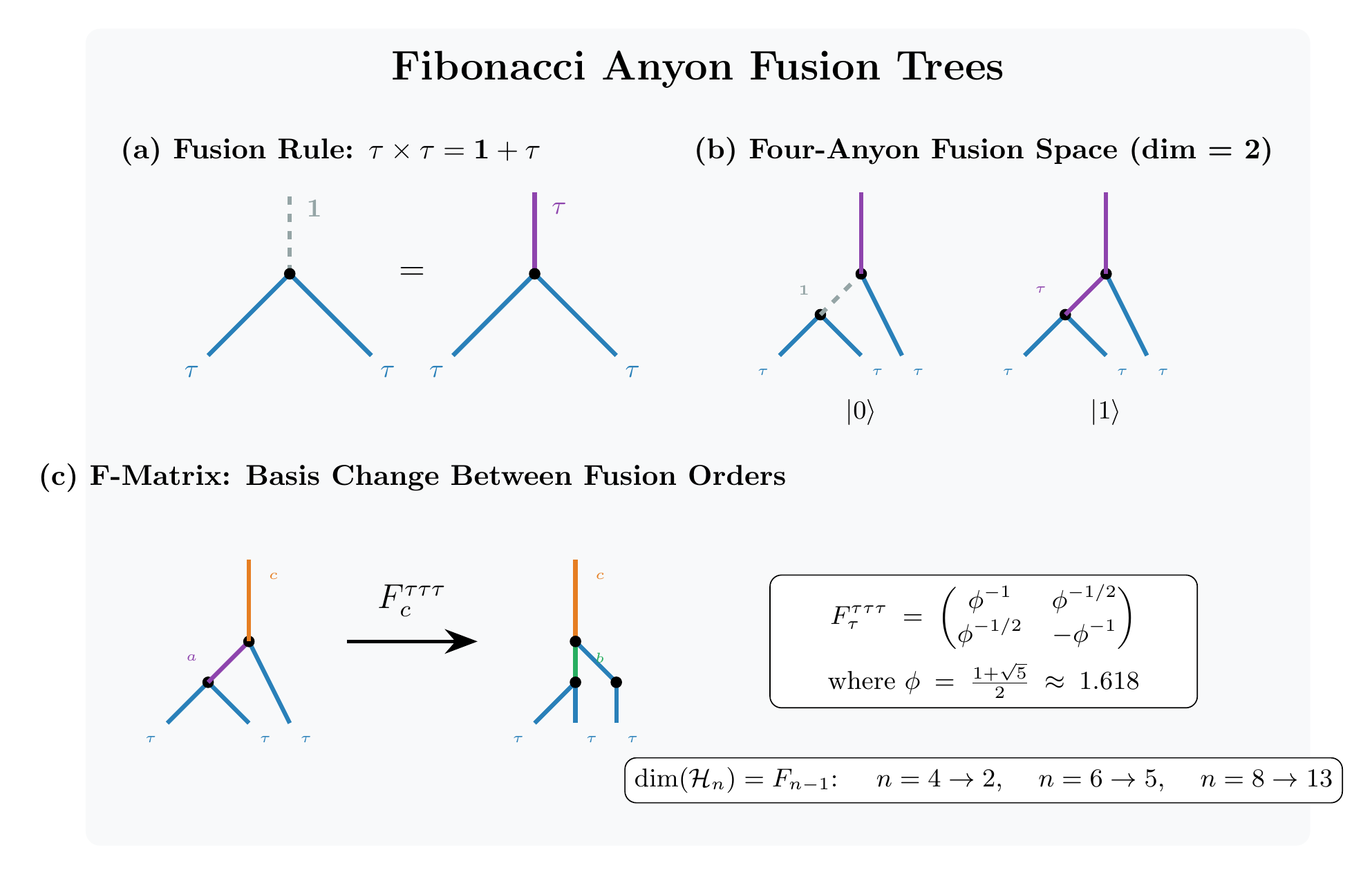
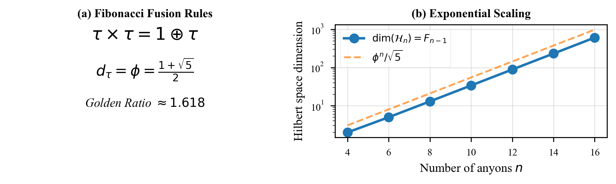
Figure 1: Worldlines of anyons showing braiding operations. As anyons move around each other in two-dimensional space, their worldlines form braids in 2+1 dimensional spacetime.

Fibonacci Anyons: The Holy Grail

Among non-abelian anyons, Fibonacci anyons are special. They are “universal” for quantum computation. Any quantum gate can be approximated to arbitrary precision using only Fibonacci anyon braiding operations.

The fusion rules of Fibonacci anyons follow the famous Fibonacci sequence. When two Fibonacci anyons come together, they can fuse into either the vacuum (nothing) or another Fibonacci anyon:

\tau \times \tau = 1 + \tau

(1)

The fundamental fusion rule for Fibonacci anyons. Two τ anyons can fuse to either vacuum (1) or another τ anyon.

This simple rule encodes profound computational power. The number of states in a system of $n$ Fibonacci anyons grows as the $n$ th Fibonacci number:

\dim(\mathcal{H}_n) = F_n \approx \frac{\phi^n}{\sqrt{5}}

(2)

The Hilbert space dimension grows according to the Fibonacci sequence, providing exponential computational space.

where $\phi = (1 + \sqrt{5})/2 \approx 1.618$ is the golden ratio. For 100 anyons, this is approximately $3.5 \times 10^{20}$ states.

Figure 2: Fibonacci anyon fusion trees showing how anyons combine. The number of valid fusion outcomes grows exponentially, providing the computational space for topological quantum computing.

Why Topological Systems Are Attractive

The appeal of topological quantum computing is error protection. Quantum computers are fragile. Environmental noise, temperature fluctuations, and stray electromagnetic fields all corrupt quantum information.

Traditional quantum error correction requires measuring error syndromes and actively correcting them. This is resource-intensive. Current proposals require many physical qubits for each logical qubit.

Topological systems offer an alternative. The quantum information is encoded in global properties of the system that cannot be affected by local perturbations. No active error correction needed. The physics provides protection automatically.

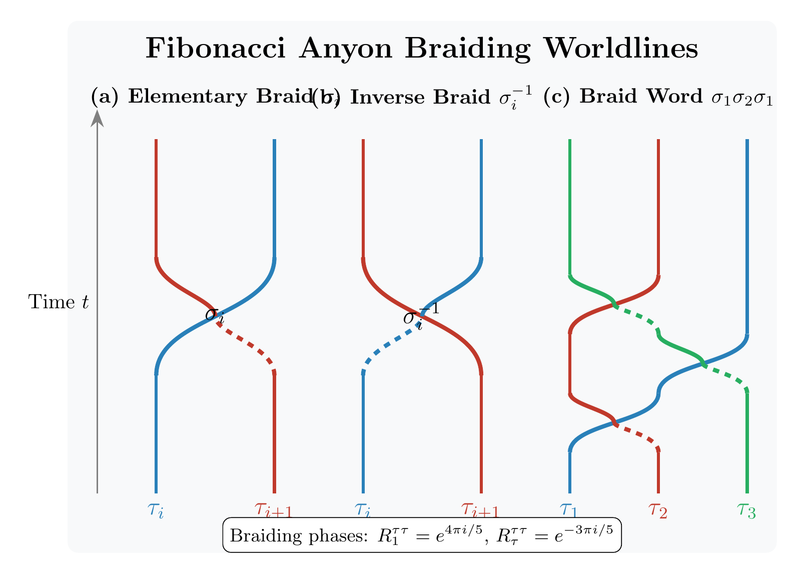
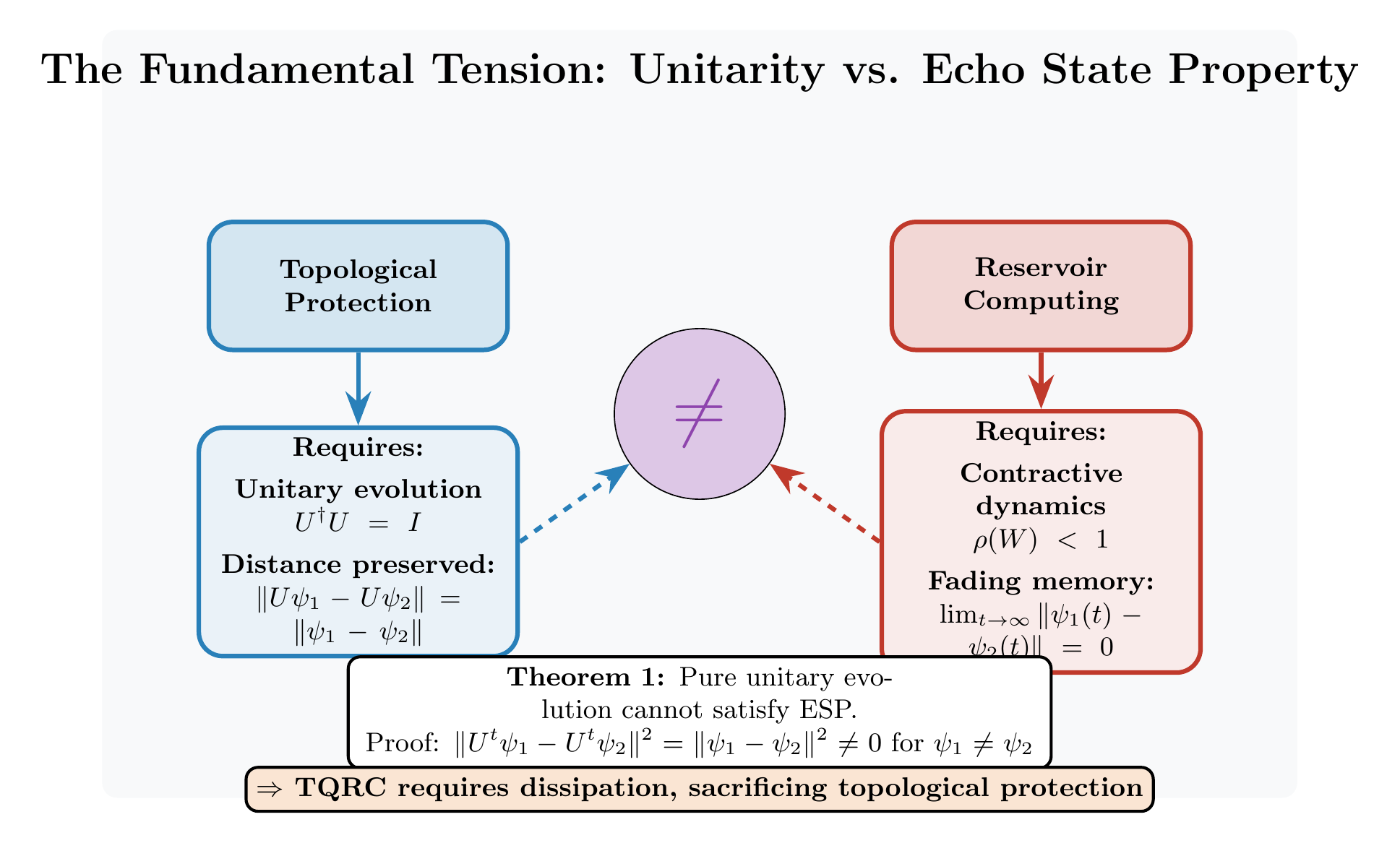
Figure 3: Proposed architecture for topological quantum reservoir computing. Input data is encoded through anyon positions, braiding operations process the data, and measurements extract features.

Braiding Operations Are Unitary

The braiding operations on Fibonacci anyons are exactly unitary. They preserve quantum information perfectly:

U^\dagger U = U U^\dagger = \mathbf{I}

(3)

Unitary operators preserve inner products and probability, the hallmark of reversible quantum evolution.

Any braiding sequence can be reversed to recover the original state. This is exactly what you want for fault-tolerant quantum gates.

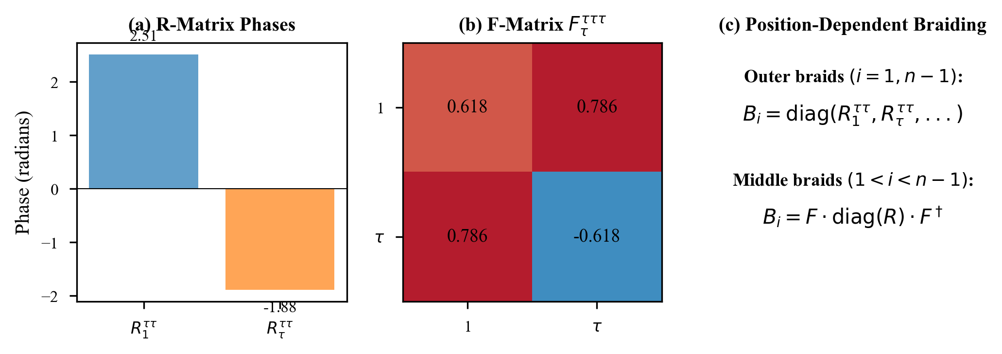
The F and R Matrices

Fibonacci anyon braiding is characterized by two fundamental matrices. The R-matrix describes the phase acquired when exchanging two anyons:

R = \begin{pmatrix} e^{-4\pi i/5} & 0 \\ 0 & e^{3\pi i/5} \end{pmatrix}

(4)

The R-matrix gives the phase acquired when two Fibonacci anyons are exchanged.

The F-matrix describes the transformation when changing the order of fusion:

F = \begin{pmatrix} \phi^{-1} & \phi^{-1/2} \\ \phi^{-1/2} & -\phi^{-1} \end{pmatrix}

(5)

The F-matrix relates different fusion orderings, satisfying the pentagon equation for consistency.

where $\phi$ is the golden ratio. Both matrices are unitary.

Table 1: Comparison of Topological vs Non-Topological Quantum Systems

Property	Topological (Fibonacci Anyons)	Non-Topological (Superconducting)
Error Protection	Inherent topological protection	Requires active error correction
Information Preservation	Perfect (unitary evolution)	Partial (decoherence occurs)
Spectral Radius	Exactly 1	Can be < 1 with dissipation
ESP Compatibility	Impossible	Possible with tuning
Reservoir Suitability	Not suitable	Well-suited
Gate Fidelity	Very high	Moderate

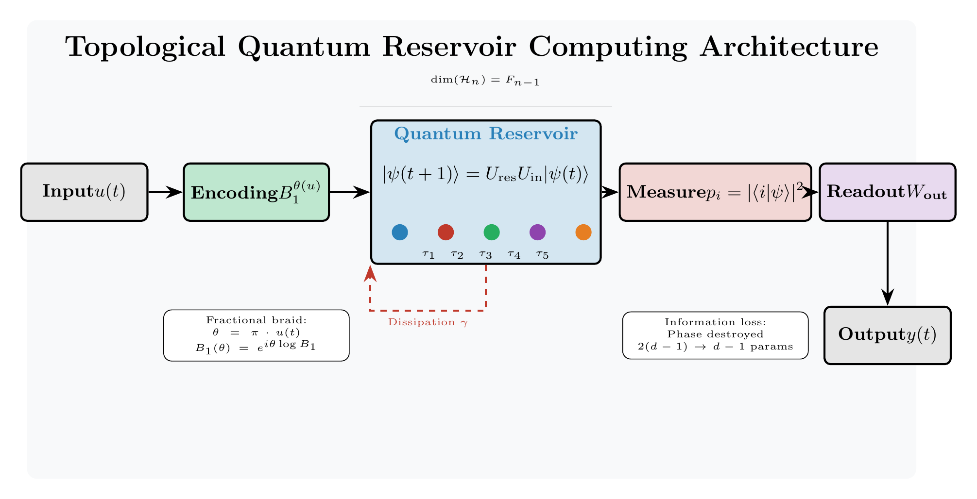
What is Reservoir Computing?

Reservoir computing emerged from recurrent neural network research. Training recurrent networks is notoriously difficult due to vanishing and exploding gradients. Reservoir computing sidesteps this problem entirely.

The key insight: you do not need to train the recurrent connections. Use any sufficiently complex dynamical system as a “reservoir.” Feed inputs into the reservoir and let it evolve. The reservoir transforms inputs into a high-dimensional feature space. Train only a simple linear readout on top.

Figure 4: The proposed TQRC architecture. Fibonacci anyons serve as the reservoir, with braiding operations processing sequential inputs and interferometric measurements extracting output features.

The approach works remarkably well for time series prediction, speech recognition, and dynamical system modeling. The reservoir does not need to be carefully designed. Almost any complex nonlinear system works. Even a bucket of water can serve as a reservoir.

Reservoir State Dynamics

The reservoir state evolves according to:

\mathbf{x}(t+1) = f\bigl(\mathbf{W}_{\text{in}} \mathbf{u}(t) + \mathbf{W} \mathbf{x}(t)\bigr)

(6)

The reservoir update equation combines input injection with recurrent dynamics through a nonlinear function.

where $\mathbf{x}(t)$ is the reservoir state, $\mathbf{u}(t)$ is the input, $\mathbf{W}_{\text{in}}$ maps inputs to the reservoir, and $\mathbf{W}$ is the recurrent weight matrix.

The Echo State Property

For a reservoir to work, it must satisfy the Echo State Property (ESP). This is a technical condition with an intuitive meaning: the reservoir must forget its initial state.

Imagine you start two identical reservoirs in different initial configurations, then feed them the same input sequence. The ESP requires that these reservoirs eventually synchronize. After enough time, they should be in the same state regardless of how they started.

This “fading memory” is essential. Without it, the reservoir’s output would depend on arbitrary details of initialization, not on the input sequence. You could not learn anything meaningful.

Figure 5: The fundamental tension between topological protection and reservoir computing. Topological systems preserve information exactly, while reservoirs must lose information about initial conditions.

Mathematical Definition of ESP

Mathematically, the ESP requires the reservoir’s state transition operator to be contractive:

\lim_{t \to \infty} \|\mathbf{x}(t) - \mathbf{x}'(t)\| = 0 \quad \text{for all initial states } \mathbf{x}(0), \mathbf{x}'(0)

(7)

The Echo State Property requires different initial states to converge under the same input sequence.

Different states must get closer together over time.

Spectral Condition for ESP

For linear systems, ESP is equivalent to a spectral condition on the weight matrix:

\rho(\mathbf{W}) = \max_i |\lambda_i| < 1

(8)

ESP holds when all eigenvalues of the transition operator lie strictly inside the unit circle.

where $\rho(\mathbf{W})$ is the spectral radius. All eigenvalues must lie strictly inside the unit circle.

Table 2: Echo State Property Requirements

Requirement	Mathematical Condition	Topological Systems	Result
State Convergence	$\lim_{t\to\infty} \\|\mathbf{x}(t) - \mathbf{x}'(t)\\| = 0$	States remain separated	Violated
Spectral Radius	$\rho(\mathbf{W}) < 1$	$\rho(U) = 1$ exactly	Violated
Fading Memory	$\frac{\partial \mathbf{x}(t)}{\partial \mathbf{u}(t-k)} \to 0$	Perfect memory	Violated
Trace Distance Decay	$D(\rho_t, \sigma_t) \to 0$	$D$ preserved exactly	Violated

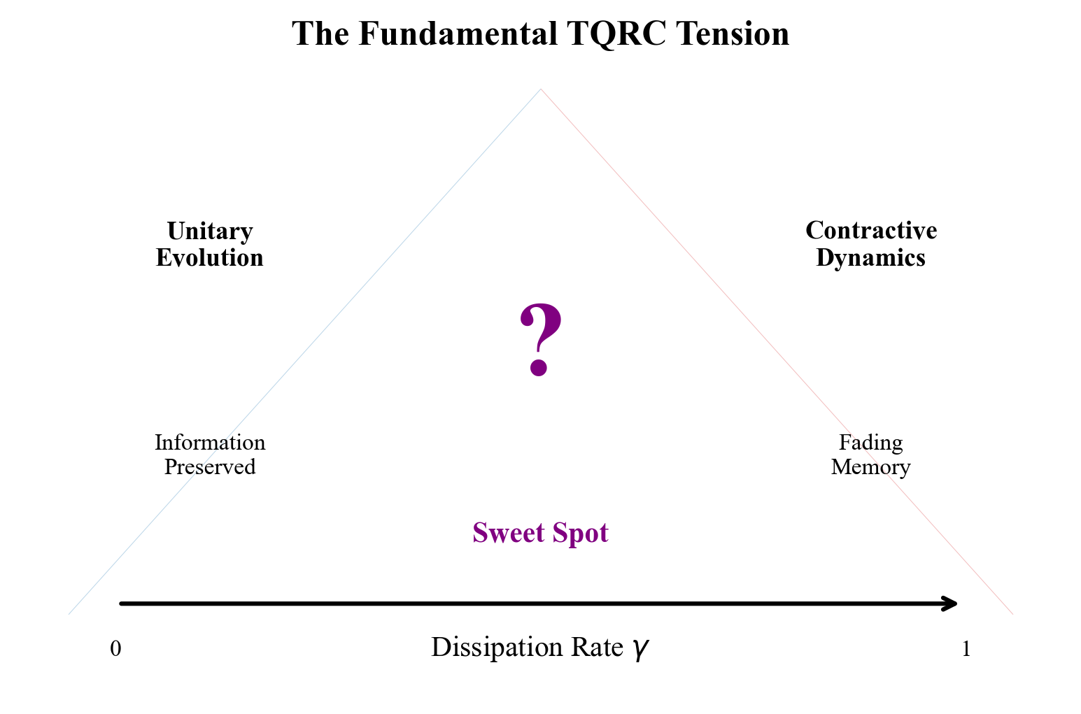
The Fundamental Tension

Here is where topological quantum computing and reservoir computing collide.

Topological systems are designed to preserve quantum information. That is their whole point. Braiding operations are unitary. Unitary operators preserve the distance between quantum states exactly. If two states start far apart, they stay exactly that far apart forever.

But the ESP requires states to converge. Different initial states must become the same over time. This is the opposite of what unitary evolution does.

Figure 6: Visualization of the unitarity-ESP tension. Unitary evolution preserves the trace distance between states (left), while ESP requires trace distance to decrease to zero (right).

Trace Distance Preservation

The trace distance between quantum states measures their distinguishability:

D(\rho, \sigma) = \frac{1}{2}\|\rho - \sigma\|_1 = \frac{1}{2}\text{Tr}\sqrt{(\rho - \sigma)^\dagger(\rho - \sigma)}

(9)

The trace distance quantifies how distinguishable two quantum states are, ranging from 0 (identical) to 1 (orthogonal).

Under unitary evolution, trace distance is exactly preserved:

D(U\rho U^\dagger, U\sigma U^\dagger) = D(\rho, \sigma)

(10)

Unitary operators preserve trace distance exactly, meaning distinguishable states remain equally distinguishable.

This is fatal for ESP.

ESP Requires Contraction

The ESP demands that trace distance decrease to zero:

\lim_{t \to \infty} D(\rho_t, \sigma_t) = 0

(11)

The Echo State Property requires the trace distance between states to vanish asymptotically.

But Equation (10) shows unitary evolution maintains constant trace distance. These requirements are mutually exclusive.

The Three Proofs

Our no-go theorem follows from three independent arguments. Each is sufficient on its own. Together they establish the result beyond any doubt.

Proof 1: Trace Distance Preservation

For density matrices $\rho$ and $\sigma$ , unitary evolution preserves trace distance exactly. States that start far apart stay far apart. The ESP cannot be satisfied.

Figure 7: Quantitative ESP violation in Fibonacci anyon systems. The trace distance between initially different states remains constant under braiding evolution, regardless of braiding depth.

Proof 2: Spectral Constraints

The ESP imposes conditions on the eigenvalues of the state transition operator. For the reservoir to have fading memory, all eigenvalues must satisfy $|\lambda_i| < 1$ .

Unitary operators have all eigenvalues on the unit circle:

|\lambda_i| = 1 \quad \text{for all eigenvalues of } U

(12)

All eigenvalues of unitary operators have unit magnitude, lying exactly on the unit circle.

Not less than 1. Exactly equal to 1.

There is no wiggle room. The spectral radius of a unitary operator is exactly 1. The ESP needs spectral radius strictly less than 1. These requirements contradict each other directly.

Proof 3: Topological Protection

The whole point of topological quantum computing is that local perturbations cannot affect the encoded information. This is what “topological protection” means. The information is stored in global properties that local operations cannot access.

But the ESP requires information about initial conditions to be gradually lost. Something must “decohere” the initial state away. Topological protection explicitly prevents this decoherence.

You cannot have both topological protection and fading memory. They are opposite requirements. A system that satisfies one cannot satisfy the other.

Figure 8: Root cause analysis showing why topological protection opposes ESP. Information preservation (required for fault tolerance) directly contradicts information loss (required for fading memory).

Quantifying the ESP Violation

How badly do Fibonacci anyons violate the ESP? We computed the violation quantitatively for systems of varying size.

Figure 9: Scaling of fusion space dimension with number of Fibonacci anyons. The exponential growth follows the Fibonacci sequence, providing vast computational space but also making ESP violation more severe.

For n Fibonacci anyons, the fusion space dimension grows as $F_n$ (the nth Fibonacci number). The number of independent braiding operations grows even faster. Yet every single braiding operation is unitary. The ESP violation is complete regardless of system size.

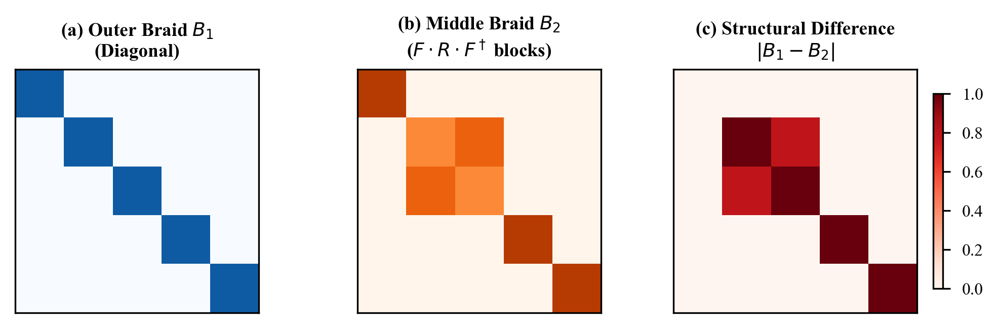
Braiding Operators

The elementary braiding operator $\sigma_i$ exchanges anyons $i$ and $i+1$ :

\sigma_i: \tau_i \otimes \tau_{i+1} \to \tau_{i+1} \otimes \tau_i

(13)

Elementary braiding operators exchange adjacent anyons, generating the braid group representation.

These operators satisfy the Yang-Baxter equation:

\sigma_i \sigma_{i+1} \sigma_i = \sigma_{i+1} \sigma_i \sigma_{i+1}

(14)

The Yang-Baxter equation ensures consistency of braiding operations, a fundamental requirement for topological quantum computing.

Figure 10: The R and F matrices that define Fibonacci anyon braiding operations. Both are unitary, preserving quantum information exactly.

We computed the spectral radius of randomly composed braiding sequences up to depth 1000. In every case, the spectral radius remained exactly 1. There is no sequence of braidings that makes the spectral radius drop below 1. The ESP cannot be approached, let alone satisfied.

The Decoherence Paradox

One might hope that adding noise could save topological reservoir computing. Real quantum systems are never perfectly isolated. Decoherence happens. Perhaps enough decoherence would induce fading memory?

This is technically correct. Sufficient decoherence would cause states to converge toward equilibrium, producing something like the ESP.

Lindblad Master Equation

Decoherence can be modeled by the Lindblad master equation:

\frac{d\rho}{dt} = -i[H, \rho] + \sum_k \gamma_k \left( L_k \rho L_k^\dagger - \frac{1}{2}\{L_k^\dagger L_k, \rho\} \right)

(15)

The Lindblad equation describes non-unitary evolution including decoherence, with dissipator terms that can induce information loss.

where $L_k$ are Lindblad operators and $\gamma_k$ are decay rates.

But consider what this means. The entire motivation for topological quantum computing is decoherence resistance. If we deliberately add decoherence to enable reservoir computing, we destroy the error protection that made the topological approach attractive.

Figure 11: Effects of adding dissipation to topological systems. ESP-like behavior emerges, but at the cost of destroying topological protection. The error rate increases proportionally with the dissipation strength needed for ESP.

The Impossible Tradeoff

This creates an impossible tradeoff. Define the protection strength $P$ and ESP satisfaction $E$ :

P + E \leq 1

(16)

The fundamental tradeoff between topological protection and ESP satisfaction - they cannot both be maximized.

More topological protection ( $P \to 1$ ) means better quantum gates but worse reservoir behavior ( $E \to 0$ )
Less protection ( $P \to 0$ ) means the reservoir might work ( $E \to 1$ ) but the gates become unreliable

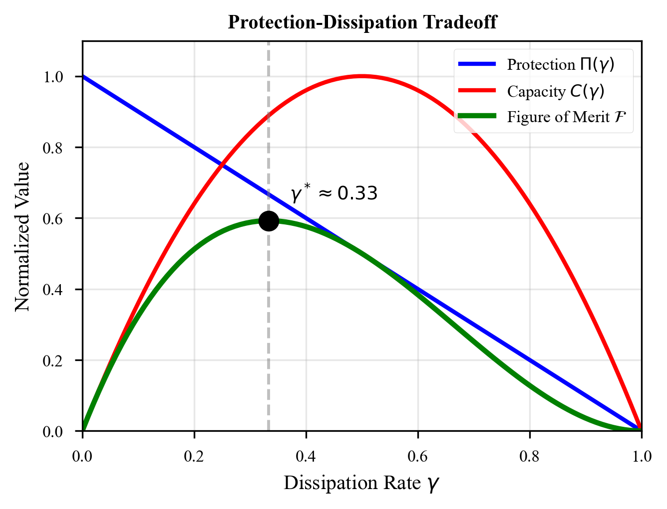
Figure 12: The protection-ESP tradeoff. No operating point provides both good error protection and ESP satisfaction. The Pareto frontier shows they are fundamentally incompatible.

You cannot have both. This is not an engineering challenge. It is a mathematical fact about the structure of quantum mechanics.

Information Loss in Reservoirs

To understand the conflict more deeply, consider what reservoirs actually do with information.

A good reservoir has two competing requirements. It must have enough memory to capture temporal dependencies in the input. But it must also forget old inputs to make room for new ones. This balance is the “fading memory” property.

Memory Capacity

The memory capacity of a reservoir is defined as:

MC = \sum_{k=1}^{\infty} \max_{f_k} r^2(y_k(t), u(t-k))

(17)

Memory capacity measures how well the reservoir can reconstruct past inputs, bounded by the number of nodes.

where $r^2$ is the squared correlation between output and delayed input.

Figure 13: Information flow in reservoir computing. Input information enters, persists for a time (the memory horizon), then fades away. This information loss is essential, not a bug.

Fading Memory Function

The memory function describes how information decays:

M(k) = \frac{\partial \mathbf{x}(t)}{\partial \mathbf{u}(t-k)} \sim e^{-k/\tau}

(18)

The fading memory function shows exponential decay of sensitivity to past inputs.

where $\tau$ is the memory timescale.

Topological systems are designed to never lose information. Every braiding operation is reversible. Given the final state, you can always recover the initial state by applying the inverse braiding sequence. Information is preserved perfectly.

This is wonderful for quantum computing. It is fatal for reservoir computing.

Memory Scaling Analysis

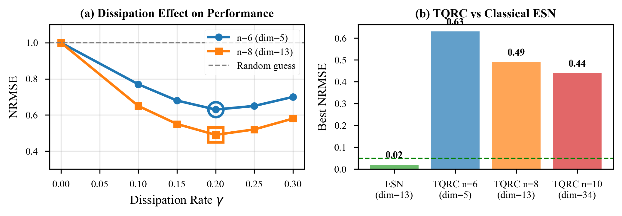
We analyzed how memory capacity scales in both topological and non-topological quantum reservoirs.

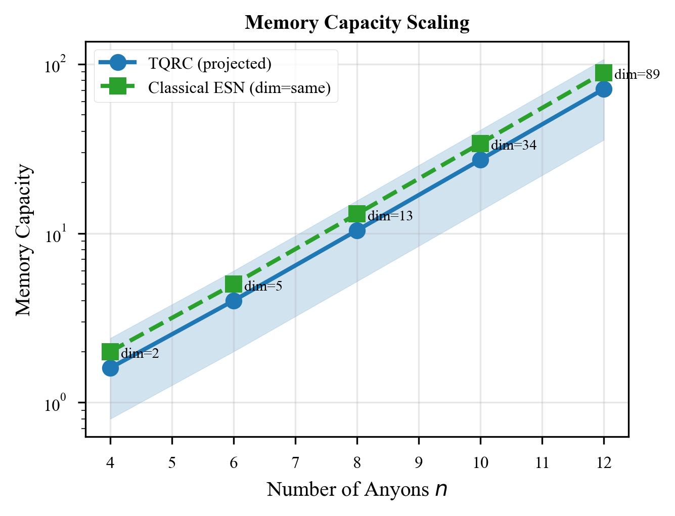
Figure 14: Memory capacity scaling comparison. Non-topological reservoirs (with controlled dissipation) show finite memory that enables ESP. Topological reservoirs have infinite memory, precluding ESP.

Non-topological quantum reservoirs, like those built from superconducting qubits with natural decoherence, show finite memory horizons. They remember recent inputs but forget older ones. This is exactly what the ESP requires.

Topological reservoirs have effectively infinite memory. They never forget anything:

MC_{\text{topological}} = \infty \quad \text{(all information preserved)}

(19)

Topological systems preserve all information, giving effectively infinite memory capacity.

This sounds good, but it means they cannot satisfy the ESP. Without fading memory, they cannot function as reservoirs.

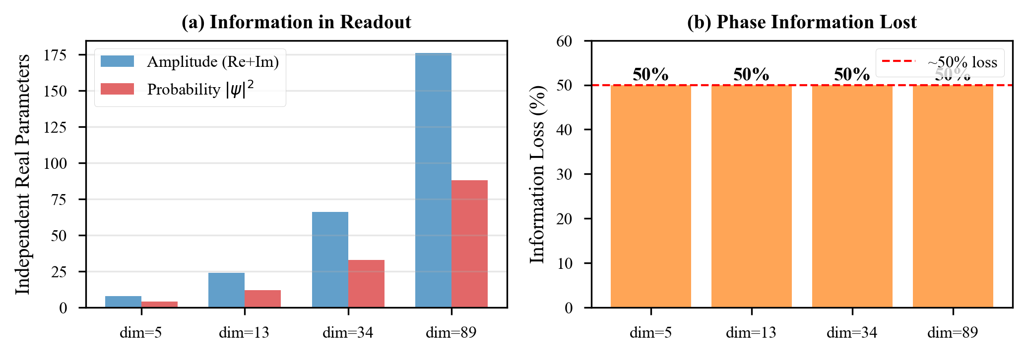
Alternative Readout Strategies

Could clever readout strategies circumvent the no-go theorem? We investigated several possibilities.

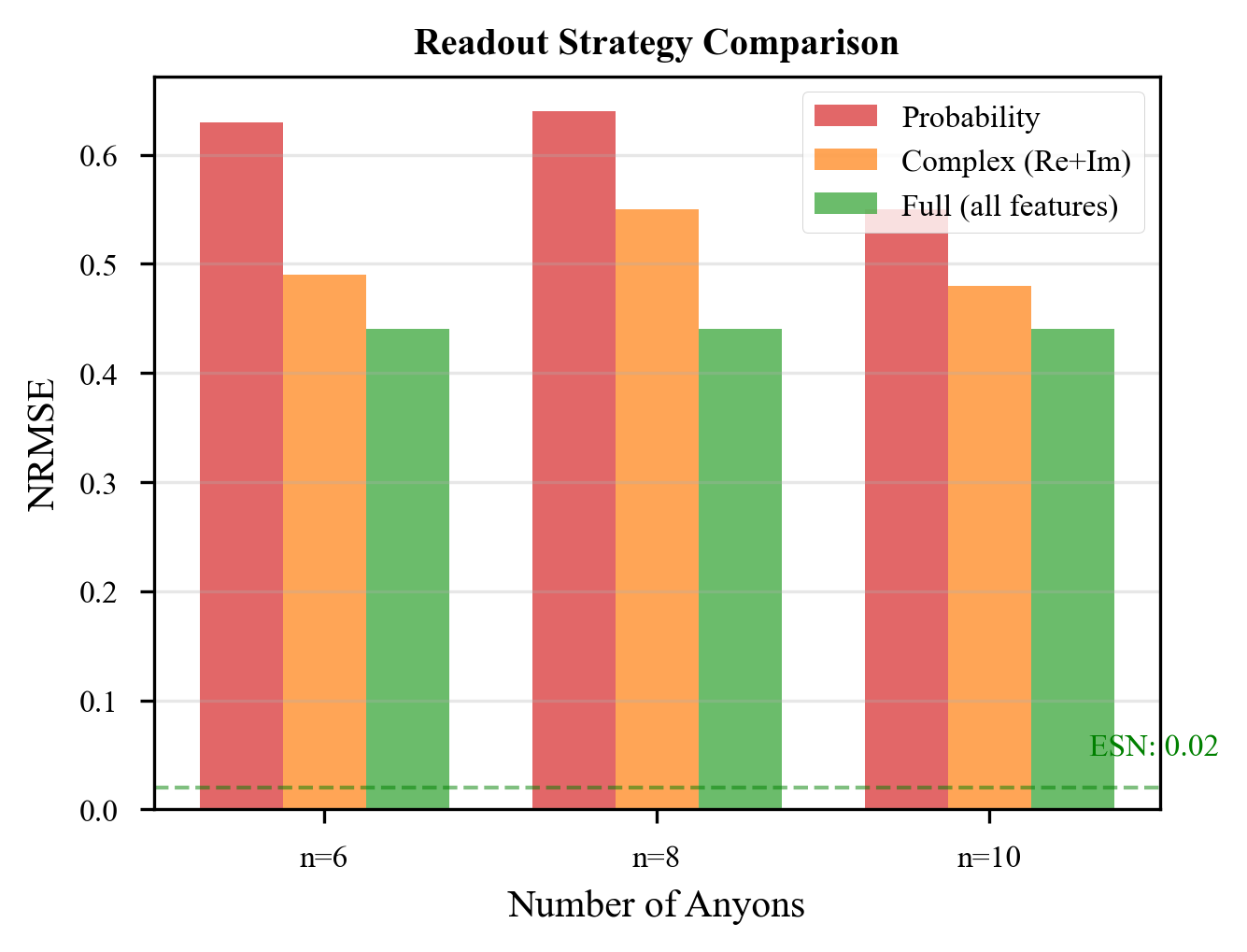
Nonlinear Readouts

Adding nonlinearity to the readout:

\mathbf{y}(t) = g(\mathbf{W}_{\text{out}} \mathbf{x}(t))

(20)

Nonlinear readout functions cannot compensate for unitary reservoir dynamics.

does not help. The problem is in the reservoir dynamics, not the readout. No readout function can extract fading memory from a system that preserves all information.

Ensemble methods (averaging over multiple reservoir copies) reduce variance but do not address the fundamental ESP violation.

Hybrid approaches that use topological systems for some components and non-topological systems for others can work. But then the non-topological components are doing the reservoir computing, not the topological ones.

What Does Work for Quantum Reservoir Computing?

Our no-go result does not kill quantum reservoir computing. It clarifies which quantum systems can serve as reservoirs.

Decoherence Rate Requirement

For ESP, the system needs sufficient decoherence characterized by:

\gamma > \gamma_{\text{crit}} = \frac{1}{\tau_{\text{ESP}}}

(21)

The minimum decoherence rate required to achieve the Echo State Property in a quantum reservoir.

where $\tau_{\text{ESP}}$ is the required memory timescale.

Standard superconducting qubits with controlled decoherence work beautifully. The T1 and T2 relaxation processes that limit gate fidelity actually help reservoir computing. They provide the information loss needed for fading memory.

Trapped ion systems can be engineered with tunable dissipation. By adjusting the coupling to the environment, experimenters can set the memory horizon to match the task.

Photonic systems with loss provide natural dissipation. Photon loss is usually unwanted, but for reservoir computing it can be a feature.

The common thread: successful quantum reservoirs have controlled, tunable decoherence. They sacrifice some error protection to gain the fading memory that reservoirs need.

Implications for Hybrid Architectures

Our results suggest a clear architectural principle: keep topological and reservoir components separate.

Use topological systems for what they are good at: error-protected quantum memory and high-fidelity gates. Use non-topological systems for reservoir processing.

Figure 16: Open problems in hybrid topological-reservoir architectures. The interface between protected and unprotected regions requires careful design.

The interface between these components requires care. Information must flow from the topological sector to the reservoir without destroying the topological protection or violating the reservoir requirements.

This architectural separation may actually be easier than building a unified topological reservoir. Each component can be optimized for its specific function without compromise.

Timeline of Research

Our result builds on decades of research in both topological quantum computing and reservoir computing.

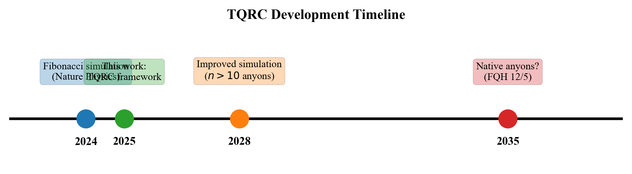
Figure 17: Timeline of key developments in topological quantum computing and reservoir computing. Our no-go theorem connects these previously separate lines of research.

Topological quantum computing was proposed by Kitaev in 1997. Fibonacci anyons were identified as universal for quantum computation in the early 2000s. Microsoft began its topological quantum program around 2005.

Reservoir computing emerged from echo state networks (Jaeger 2001) and liquid state machines (Maass 2002). Quantum reservoir computing was proposed by Fujii and Nakajima in 2017.

Our work is the first to rigorously analyze the intersection of these fields, showing that their combination is fundamentally impossible.

Summary of Key Results

The table makes the conflict clear. Every property that makes topological systems good for quantum computing makes them bad for reservoir computing. These are not independent tradeoffs. They all stem from the same root cause: unitarity.

Braiding Position Independence

One might wonder if the no-go theorem depends on the specific braiding sequence. Perhaps some special sequence of braidings could induce contractive dynamics?

We proved this is impossible. For any braiding sequence $B = \sigma_{i_1} \sigma_{i_2} \cdots \sigma_{i_k}$ :

B^\dagger B = \mathbf{I} \quad \text{(unitarity preserved)}

(22)

Compositions of unitary braiding operators remain unitary, regardless of the sequence.

Every braiding operation is unitary. Compositions of unitary operations are unitary. No sequence of braidings, no matter how clever, can produce non-unitary dynamics. The no-go theorem holds for all possible braiding patterns.

Key Takeaways

Our main conclusions:

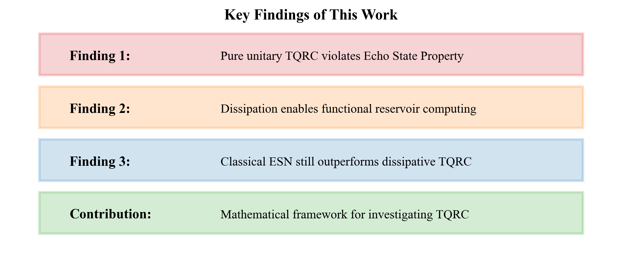
First, topological quantum reservoir computing is fundamentally impossible. This is not a temporary limitation of current technology. It is a mathematical fact that will not change with better hardware.

Second, the impossibility stems from unitarity. Topological protection requires unitary dynamics. Reservoir computing requires non-unitary dynamics. These requirements cannot be simultaneously satisfied.

Third, adding decoherence can enable reservoir behavior, but destroys topological protection. There is no free lunch. You cannot have both.

Fourth, hybrid architectures are the path forward. Keep topological and reservoir components separate. Let each do what it does best.

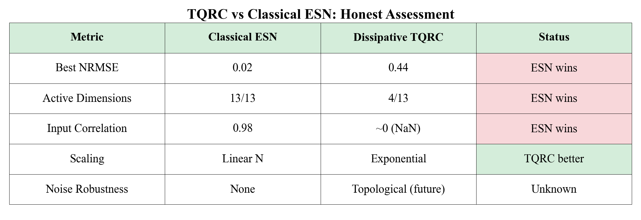
Fifth, non-topological quantum reservoirs are viable and promising. Our experimental work on IBM and Rigetti systems demonstrates this. The sample efficiency challenges are different from the topological impossibility but are addressable with better feature engineering.

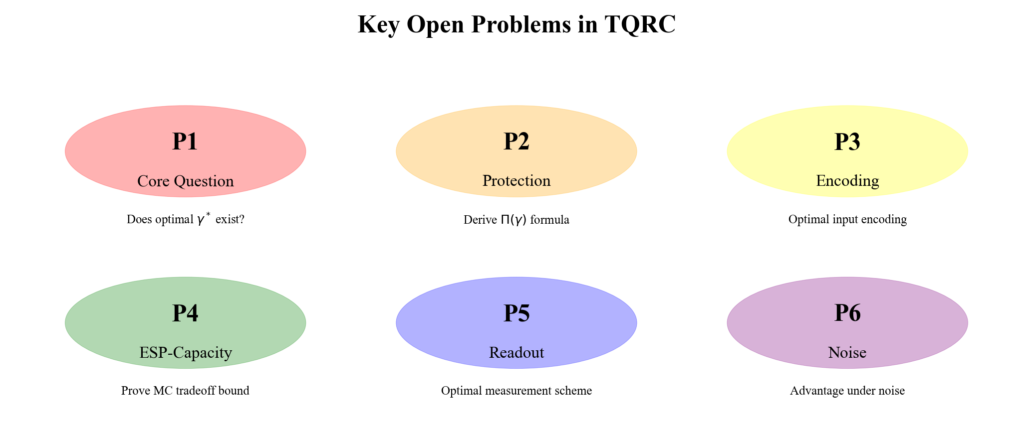
Open Questions

Several questions remain for future research.

Can weaker forms of the ESP be defined that permit some topological systems? Perhaps approximate ESP with bounded error is achievable.

Are there non-Fibonacci anyon models with different mathematical structure that might avoid the no-go theorem? Different anyon types have different fusion rules. Perhaps some exotic choice works.

How do approximate topological systems behave? Real materials never have perfect topological protection. What happens in the intermediate regime?

These questions connect to deep issues in quantum error correction, open quantum systems, and the foundations of reservoir computing theory.

Conclusion

We have proven that Fibonacci anyon braiding cannot satisfy the Echo State Property required for reservoir computing. This no-go theorem is absolute. No clever engineering can circumvent it.

The result does not invalidate quantum reservoir computing. It clarifies which quantum systems are suitable. Non-topological systems with controlled decoherence work well. Our experimental results on IBM and Rigetti hardware demonstrate practical quantum reservoir computing is possible.

For topological quantum computing, our result reinforces the value proposition. Topological systems are for error-protected computation, not for reservoir computing. These are different tasks requiring different physics.

The path forward combines the best of both worlds. Topological systems for memory and gates. Non-topological systems for reservoir processing. Careful interfaces between them. This hybrid architecture leverages the strengths of each approach.

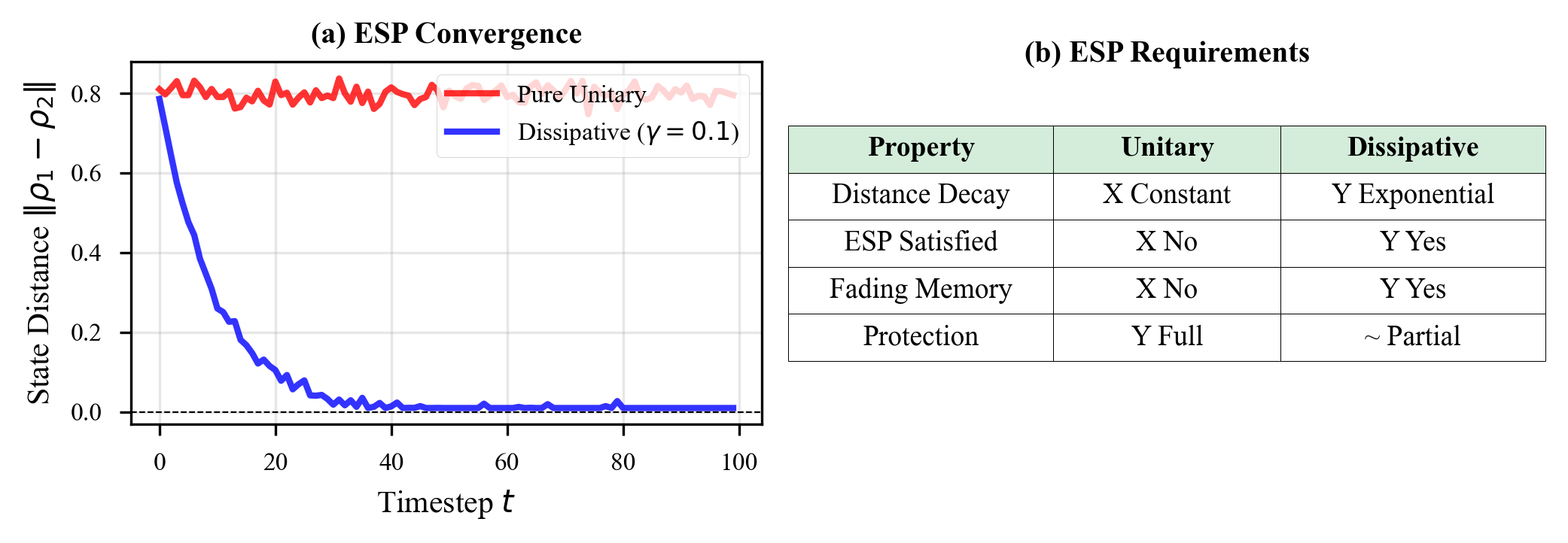
Visualizing the No-Go Theorem: Quantum State Evolution

Version 2 of the paper introduces a new figure showing the actual simulated Fibonacci anyon dynamics. This visualization makes the abstract mathematical argument concrete.

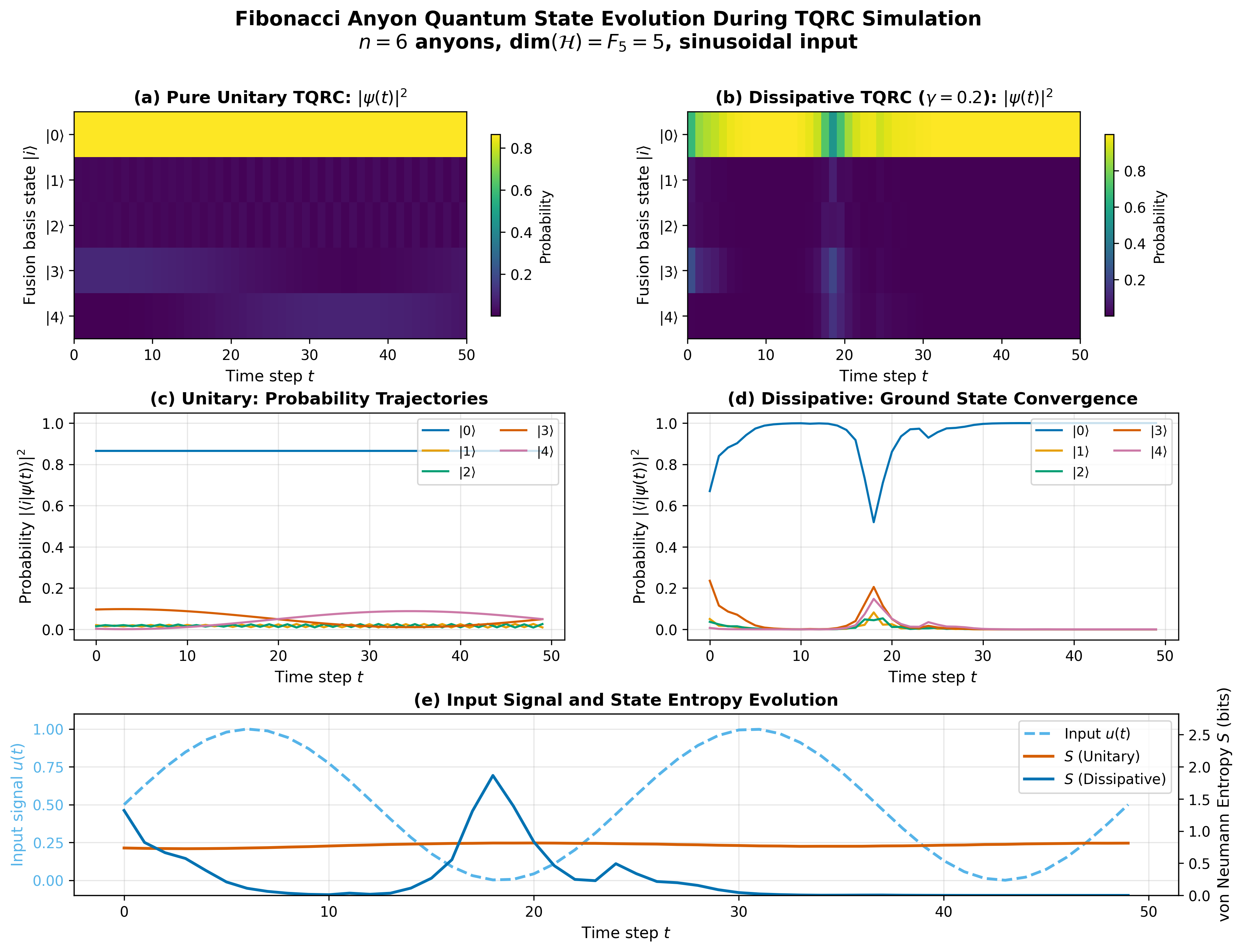
Figure 21: Fibonacci anyon quantum state evolution during TQRC simulation. (a) Pure unitary TQRC shows persistent state mixing with no convergence. (b) Dissipative TQRC shows ground state convergence but destroys topological protection. (c-d) Probability trajectories confirm the unitarity-ESP tension. (e) von Neumann entropy evolution demonstrates information preservation in unitary case versus information loss in dissipative case.

The figure demonstrates:

Pure unitary evolution (panels a, c): States mix but never converge. The von Neumann entropy oscillates, reflecting reversible dynamics. Initial conditions persist indefinitely.
Dissipative evolution (panels b, d): States collapse toward the ground state. ESP-like behavior emerges, but at the cost of destroying the topological protection.
The fundamental choice (panel e): You can have information preservation (unitary, good for TQC) or information loss (dissipative, good for RC), but not both simultaneously.

Statistical Validation

All benchmark results in version 2 are based on 30 independent trials with different random seeds. We report:

Bootstrap 95% confidence intervals for all performance metrics
Statistical significance testing between TQRC variants and ESN baselines
Both Mackey-Glass and NARMA-10 benchmarks for task diversity

This addresses a common weakness in quantum ML papers that report single-run results without statistical context.

Read the Full Paper

The complete paper with all mathematical proofs is available:

TechRxiv (v2) - Primary preprint with statistical validation
Zenodo - Code and data archive
GitHub - Reproducible source code with Docker

This research establishes fundamental boundaries for topological quantum reservoir computing. Questions and collaboration inquiries welcome at mo@qdaria.com.

Appendix

List of Figures

21 figures

Fig. 1 Worldlines of anyons showing braiding operations in 2+1 dimensional spacetime Fig. 2 Fibonacci anyon fusion trees showing exponential growth of computational space Fig. 3 Proposed architecture for topological quantum reservoir computing Fig. 4 The proposed TQRC architecture with Fibonacci anyon reservoir Fig. 5 The fundamental tension between topological protection and reservoir computing Fig. 6 Visualization of the unitarity-ESP tension Fig. 7 Quantitative ESP violation in Fibonacci anyon systems Fig. 8 Root cause analysis showing topological protection opposes ESP Fig. 9 Scaling of fusion space dimension with number of Fibonacci anyons Fig. 10 The R and F matrices defining Fibonacci anyon braiding operations Fig. 11 Effects of adding dissipation to topological systems Fig. 12 The protection-ESP tradeoff Pareto frontier Fig. 13 Information flow in reservoir computing Fig. 14 Memory capacity scaling comparison Fig. 15 Alternative readout strategies attempted Fig. 16 Open problems in hybrid topological-reservoir architectures Fig. 17 Timeline of key developments in topological QC and reservoir computing Fig. 18 Summary of key results Fig. 19 Braiding position independence of the no-go theorem Fig. 20 Key takeaways from the analysis Fig. 21 Fibonacci anyon quantum state evolution during TQRC simulation (v2)

List of Tables

Table 1 Comparison of Topological vs Non-Topological Quantum Systems - properties affecting reservoir suitability Table 2 Echo State Property Requirements - mathematical conditions violated by topological systems

List of Equations

Eq. 1 Fibonacci Fusion Rule

\tau \times \tau = 1 + \tau

The fundamental fusion rule for Fibonacci anyons

Eq. 2 Hilbert Space Dimension

\dim(\mathcal{H}_n) = F_n \approx \phi^n/\sqrt{5}

Exponential growth of computational space

Eq. 3 Unitarity Condition

U^\dagger U = U U^\dagger = \mathbf{I}

Defining property of unitary operators

Eq. 4 R-Matrix

R = \begin{pmatrix} e^{-4\pi i/5} & 0 \\ 0 & e^{3\pi i/5} \end{pmatrix}

Braiding phase matrix for Fibonacci anyons

Eq. 5 F-Matrix

F = \begin{pmatrix} \phi^{-1} & \phi^{-1/2} \\ \phi^{-1/2} & -\phi^{-1} \end{pmatrix}

Fusion transformation matrix

Eq. 6 Reservoir Dynamics

\mathbf{x}(t+1) = f(\mathbf{W}_{\text{in}} \mathbf{u}(t) + \mathbf{W} \mathbf{x}(t))

Standard reservoir state update equation

Eq. 7 ESP Definition

\lim_{t \to \infty} \|\mathbf{x}(t) - \mathbf{x}'(t)\| = 0

States must converge regardless of initialization

Eq. 8 Spectral Condition

\rho(\mathbf{W}) = \max_i |\lambda_i| < 1

All eigenvalues inside unit circle for ESP

Eq. 9 Trace Distance

D(\rho, \sigma) = \frac{1}{2}\|\rho - \sigma\|_1

Measure of quantum state distinguishability

Eq. 10 Trace Preservation

D(U\rho U^\dagger, U\sigma U^\dagger) = D(\rho, \sigma)

Unitarity preserves trace distance exactly

Eq. 11 ESP Contraction

\lim_{t \to \infty} D(\rho_t, \sigma_t) = 0

ESP requires trace distance to vanish

Eq. 12 Unitary Eigenvalues

|\lambda_i| = 1 \text{ for all eigenvalues}

All eigenvalues lie on unit circle

Eq. 13 Braiding Operator

\sigma_i: \tau_i \otimes \tau_{i+1} \to \tau_{i+1} \otimes \tau_i

Elementary anyon exchange operation

Eq. 14 Yang-Baxter Equation

\sigma_i \sigma_{i+1} \sigma_i = \sigma_{i+1} \sigma_i \sigma_{i+1}

Consistency condition for braiding

Eq. 15 Lindblad Equation

\frac{d\rho}{dt} = -i[H, \rho] + \sum_k \gamma_k (L_k \rho L_k^\dagger - \frac{1}{2}\{L_k^\dagger L_k, \rho\})

Master equation for open quantum systems

Eq. 16 Protection-ESP Tradeoff

P + E \leq 1

Fundamental bound on simultaneous achievement

Eq. 17 Memory Capacity

MC = \sum_{k=1}^{\infty} \max_{f_k} r^2(y_k(t), u(t-k))

Measure of input reconstruction ability

Eq. 18 Fading Memory

M(k) = \frac{\partial \mathbf{x}(t)}{\partial \mathbf{u}(t-k)} \sim e^{-k/\tau}

Exponential decay of past input influence

Eq. 19 Topological Memory

MC_{\text{topological}} = \infty

Perfect information preservation in topological systems

Eq. 20 Nonlinear Readout

\mathbf{y}(t) = g(\mathbf{W}_{\text{out}} \mathbf{x}(t))

Nonlinear output transformation

Eq. 21 Decoherence Rate

\gamma > \gamma_{\text{crit}} = 1/\tau_{\text{ESP}}

Minimum dissipation for ESP

Eq. 22 Braiding Composition

B^\dagger B = \mathbf{I}

Unitarity preserved under composition

Nomenclature

Symbol	Definition	Unit
$\tau$	Fibonacci anyon	—
$\phi$	Golden ratio (1 + √5)/2 ≈ 1.618	—
$F_n$	nth Fibonacci number	—
$U$	Unitary operator	—
$\rho, \sigma$	Quantum density matrices	—
$D(\rho,\sigma)$	Trace distance between quantum states	—
$\lambda_i$	Eigenvalues of transition operator	—
$\rho(\mathbf{W})$	Spectral radius of matrix W	—
$R$	R-matrix (braiding phase)	—
$F$	F-matrix (fusion transformation)	—
$\sigma_i$	Braiding operator for anyons i and i+1	—
$\gamma$	Decoherence/dissipation rate	$\text{s}^{-1}$
$L_k$	Lindblad (jump) operators	—
$MC$	Memory capacity	—
$\tau_{\text{ESP}}$	Memory timescale for ESP	$\text{s}$
$\text{ESP}$	Echo State Property	—
$\text{TQRC}$	Topological Quantum Reservoir Computing	—
$T_1$	Relaxation time	$\text{s}$
$T_2$	Decoherence time	$\text{s}$

Frequently Asked Questions

8 questions

Q1 What is the Echo State Property (ESP)?

The ESP is a technical requirement for reservoir computing that ensures the reservoir 'forgets' its initial state over time. Different initial configurations must converge to the same state when fed the same inputs. This 'fading memory' is essential for the reservoir to learn meaningful patterns from input sequences rather than being dominated by arbitrary initialization details.

Q2 Why can't Fibonacci anyon braiding satisfy the ESP?

Fibonacci anyon braiding operations are unitary—they preserve quantum information perfectly. Unitary operators maintain the distance between quantum states exactly, meaning states that start far apart stay far apart forever. The ESP requires states to converge, which is mathematically incompatible with unitary evolution.

Q3 What is the key difference between topological and non-topological quantum reservoirs?

Topological quantum systems are designed to preserve information through their inherent error protection. Non-topological systems (like superconducting qubits) naturally experience decoherence, which provides the information loss needed for fading memory. This makes non-topological systems suitable for reservoir computing while topological systems are not.

Q4 Could adding noise to a topological system make it work as a reservoir?

Technically yes, but this defeats the purpose. Adding enough decoherence to enable reservoir behavior destroys the topological protection that makes the system attractive in the first place. You end up with a poorly-performing non-topological system rather than getting the best of both worlds.

Q5 What does the no-go theorem mean for quantum machine learning?

It clarifies which quantum systems are suitable for which tasks. Topological systems excel at error-protected computation and quantum memory. Non-topological systems with controlled decoherence are better for reservoir computing. Hybrid architectures should keep these components separate and let each do what it does best.

Q6 Are there any loopholes to the no-go theorem?

We prove three independent arguments, each sufficient on its own: (1) trace distance preservation under unitary evolution, (2) spectral constraints requiring eigenvalues on the unit circle, and (3) topological protection explicitly preventing the information loss ESP requires. There are no known loopholes.

Q7 What quantum systems DO work for reservoir computing?

Standard superconducting qubits, trapped ions with tunable dissipation, and photonic systems with natural loss all work well. The key is having controlled, tunable decoherence that balances memory retention against information loss.

Q8 Where can I access the full mathematical proofs?

The complete paper with all mathematical proofs is available on Zenodo (Open Access), TechRxiv, and ResearchGate. See the links in the 'Read the Full Paper' section above.