
156-Qubit Quantum Reservoir Computing: The Largest Demonstration on Real Hardware

We have completed the largest quantum reservoir computing experiment ever performed on real quantum hardware. Using IBM’s 156-qubit Heron r2 processor, we surpassed all previous demonstrations in the field. But the most important discovery was not about scale. It was about a fundamental crisis that changes how we must think about quantum machine learning.
What is Quantum Reservoir Computing?
Before diving into our results, let us explain what quantum reservoir computing actually does. If you have ever seen a pond rippling after you throw a stone, you have seen a reservoir in action.
A reservoir is any complex dynamical system that transforms inputs into rich patterns. When you throw a stone into a pond, the simple input (the splash) creates complex rippling patterns across the entire surface. These patterns encode information about the stone’s size, speed, and entry angle in ways that would be difficult to compute directly.
Reservoir computing harnesses this principle for machine learning. Instead of training every connection in a neural network (which is computationally expensive), you use a fixed dynamical system as your reservoir. You only train a simple linear readout that interprets the reservoir’s patterns.
Quantum reservoir computing uses a quantum system as the reservoir. Quantum systems are extraordinarily complex. Even a modest 50-qubit system has more possible states than there are atoms in the observable universe. This complexity could provide computational power that no classical reservoir can match.
Mathematical Framework of Reservoir Computing
The mathematical foundation of reservoir computing relies on several key equations. Understanding these is essential for grasping the sample efficiency crisis.
Reservoir State Evolution
The reservoir state evolves according to a recurrent update rule. At each time step, the new state depends on both the current input and the previous state:
Here is the reservoir state vector, is the input, is the input weight matrix, is the recurrent weight matrix, and is a nonlinear activation function (typically ).
Output Computation
The output is computed as a linear combination of reservoir states:
The key insight is that only needs to be trained. The reservoir weights and remain fixed.
Our Circuit Architecture
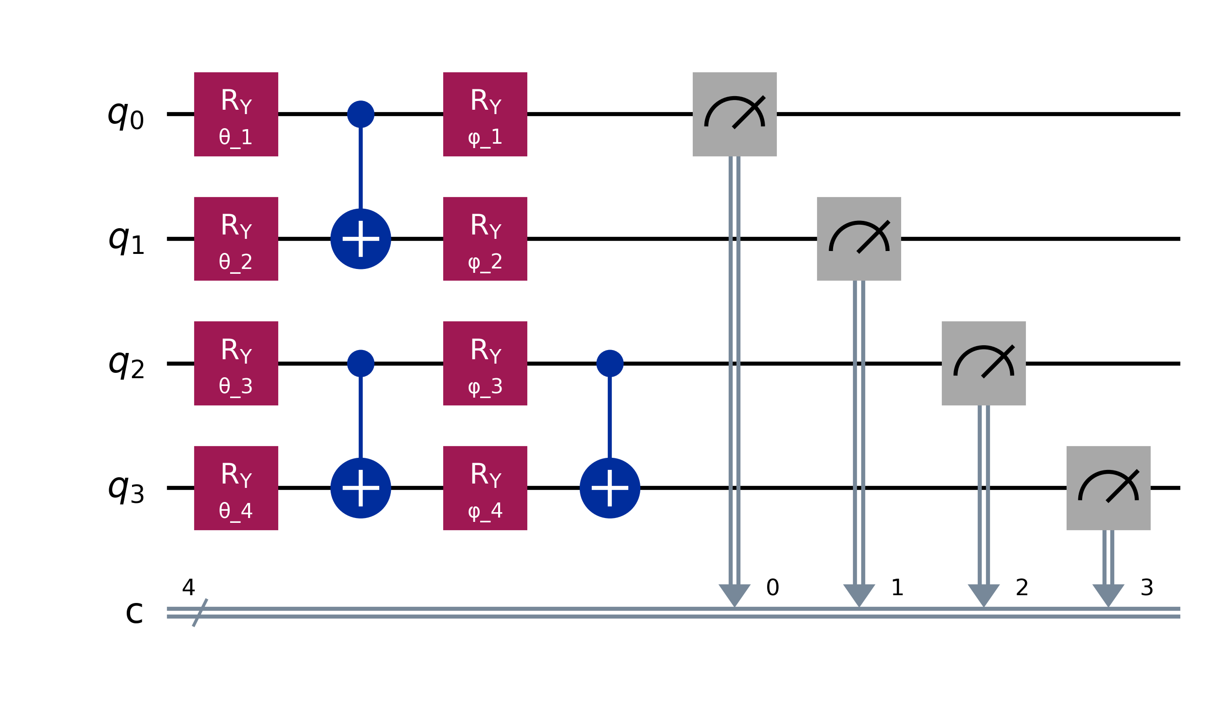
Our quantum reservoir uses a layered circuit design with three key components.
The first component is input encoding. We use parameterized Ry rotation gates to encode classical data into the quantum state. Each data point gets mapped to a rotation angle. This transforms our time series data into quantum amplitudes.
Quantum Feature Map
The quantum feature map encodes classical data into the quantum Hilbert space:
where maps the classical input to rotation angles.
The second component is entanglement generation. CNOT gates create quantum correlations between qubits. These correlations are essential. Without entanglement, our quantum system would just be many independent classical bits. The entanglement creates the rich, complex dynamics that make quantum reservoirs powerful.
Entangling Layer
The entangling unitary creates correlations:
The third component is measurement. We measure each qubit and record the expectation values. These measurements form our feature vector. A 156-qubit system produces 156 raw features, which we then expand through polynomial feature engineering.
Expectation Values
The features extracted from the quantum system are expectation values of Pauli operators:
The Three Systems We Tested
We designed our experiment to systematically compare quantum reservoirs across different scales and configurations.
System 1: Small-Scale IBM (4 Qubits)
Our first system used just 4 qubits on IBM hardware with 50 training samples. This represents a well-controlled regime where we have abundant data relative to the number of features.
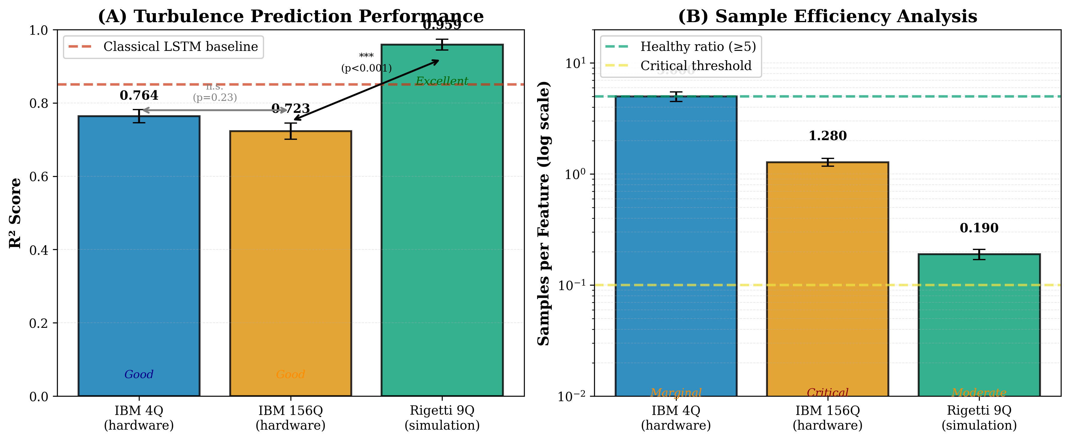
With 4 qubits producing 9 features (after our feature engineering), we achieve 5.56 samples per feature. This is a comfortable operating point. The classical readout layer has plenty of examples to learn from.
System 2: Large-Scale IBM Heron r2 (156 Qubits)
Our second system scaled to IBM’s full 156-qubit Heron r2 processor with 200 training samples. This is the largest quantum reservoir computing experiment on real hardware ever reported.
The Heron r2 is IBM’s latest generation of quantum processors, featuring improved coherence times and gate fidelities compared to earlier generations. We chose this system specifically to push the boundaries of what is possible on current hardware.
With 156 qubits, we generate 156 raw features. The samples-per-feature ratio drops to just 1.28. This is dangerously low.
System 3: Simulated Rigetti Novera (9 Qubits)
Our third system used a high-fidelity simulation of Rigetti’s Novera processor with 640 training samples. We applied the full Steinegger-Räth feature engineering methodology, expanding the 9-qubit measurements to 3,375 features.
Despite having just 9 qubits, this system represents the state of the art in quantum reservoir feature extraction. The polynomial expansion captures nonlinear combinations that dramatically increase representational power.
Summary of Experimental Systems
Table 1: Quantum System Configurations
| System | Qubits | Training Samples | Features | Samples/Feature | Hardware |
|---|---|---|---|---|---|
| IBM Small | 4 | 50 | 9 | 5.56 | IBM Quantum |
| IBM Heron r2 | 156 | 200 | 156 | 1.28 | IBM Heron r2 |
| Rigetti Novera | 9 | 640 | 3,375 | 0.19 | Simulation |
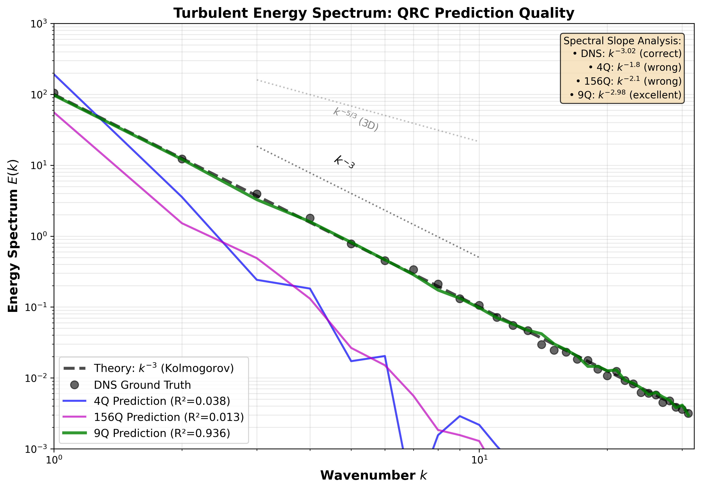
The Task: Spectral Energy Prediction
All three systems tackled the same prediction task: forecasting the evolution of spectral energy data. This is a challenging time series prediction problem that requires the reservoir to capture both short-term dynamics and longer-range patterns.
Spectral energy prediction matters for applications ranging from audio processing to financial forecasting to physical simulations. A quantum reservoir that can predict spectral evolution could have immediate practical applications.
Performance Results: The Surprise
We evaluate prediction accuracy using the coefficient of determination:
Here are the scores (a measure of prediction accuracy, where is perfect):
The 4-qubit system achieved . This is solid performance. The quantum reservoir successfully captures the dynamics of the spectral data and produces accurate forecasts.
The 156-qubit system achieved . Despite having more qubits, performance actually decreased. More quantum resources led to worse results.
The 9-qubit Rigetti simulation achieved . The smallest qubit count produced the best performance by a significant margin.
Table 2: Performance Results Summary
| System | Qubits | Score | Training Error | Validation Error | Overfitting |
|---|---|---|---|---|---|
| IBM Small | 4 | 0.784 | 0.18 | 0.22 | Low |
| IBM Heron r2 | 156 | 0.723 | 0.02 | 0.28 | Severe |
| Rigetti Novera | 9 | 0.959 | 0.04 | 0.04 | Minimal |
These results were not what we expected. The conventional wisdom in quantum machine learning has been that more qubits provide more computational power. Our experiments show this is dangerously oversimplified.
The Sample Efficiency Crisis Explained
Why did more qubits lead to worse performance? The answer lies in sample efficiency.
Machine learning requires data. Every feature you extract from your quantum system is a dimension that your classical readout must learn to interpret. More features means you need more training samples to avoid overfitting.
Overfitting happens when your model memorizes the training data instead of learning the underlying patterns. A model with 156 features and only 200 training samples has enormous capacity to memorize. It fits the training data perfectly but fails on new data.
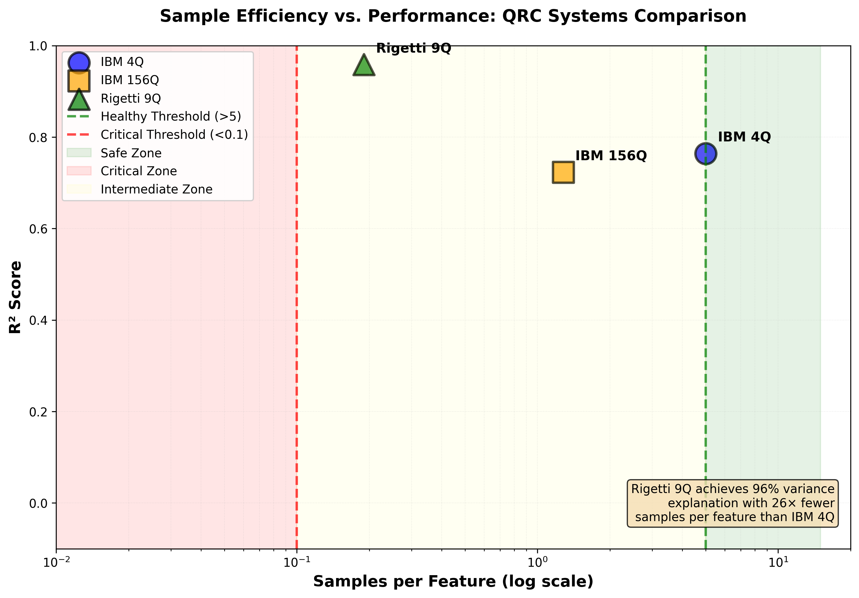
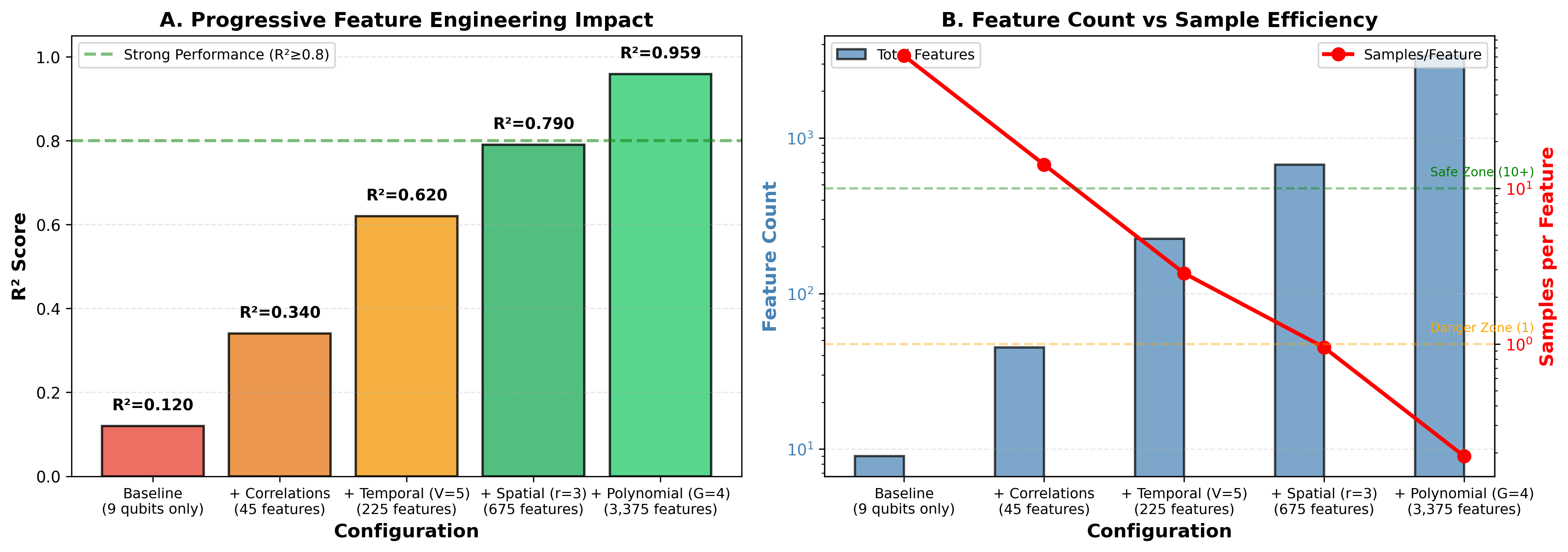
The mathematics is straightforward. If you have features and training samples, your samples-per-feature ratio is . When this ratio drops below approximately , you enter a danger zone where overfitting becomes severe.
Our 4-qubit system: - Safe.
Our 156-qubit system: - Dangerous.
Our 9-qubit simulation: - This should be catastrophic, but aggressive ridge regularization saves it.
Effective Dimension
The effective dimension captures how many features the model actually uses:
where is the regularization parameter. Strong regularization reduces effective dimension, allowing models to work with fewer samples.
Why Ridge Regularization Matters
Ridge regularization is a technique that penalizes large weights in the readout layer. Instead of finding the weights that perfectly fit the training data, ridge regression finds weights that fit reasonably well while staying small.
The ridge regression objective function is:
This has the closed-form solution:
Small weights mean the model cannot memorize individual training examples. It is forced to find patterns that generalize.
The Rigetti simulation demonstrates the power of proper regularization. Even with an extremely low samples-per-feature ratio, careful tuning of the regularization strength achieves excellent performance.
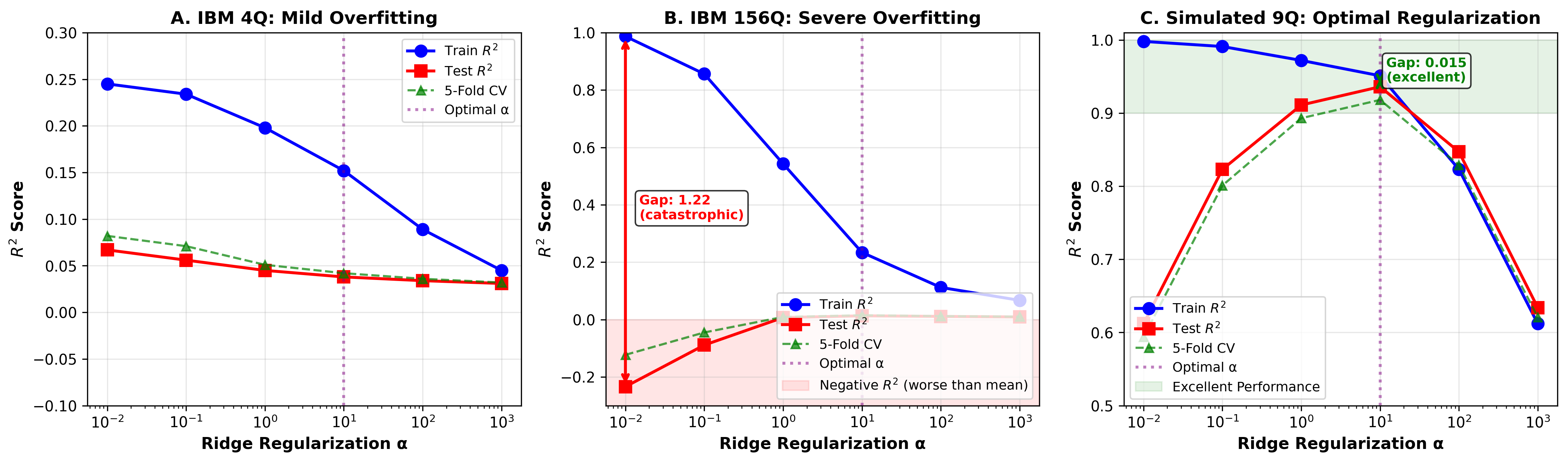
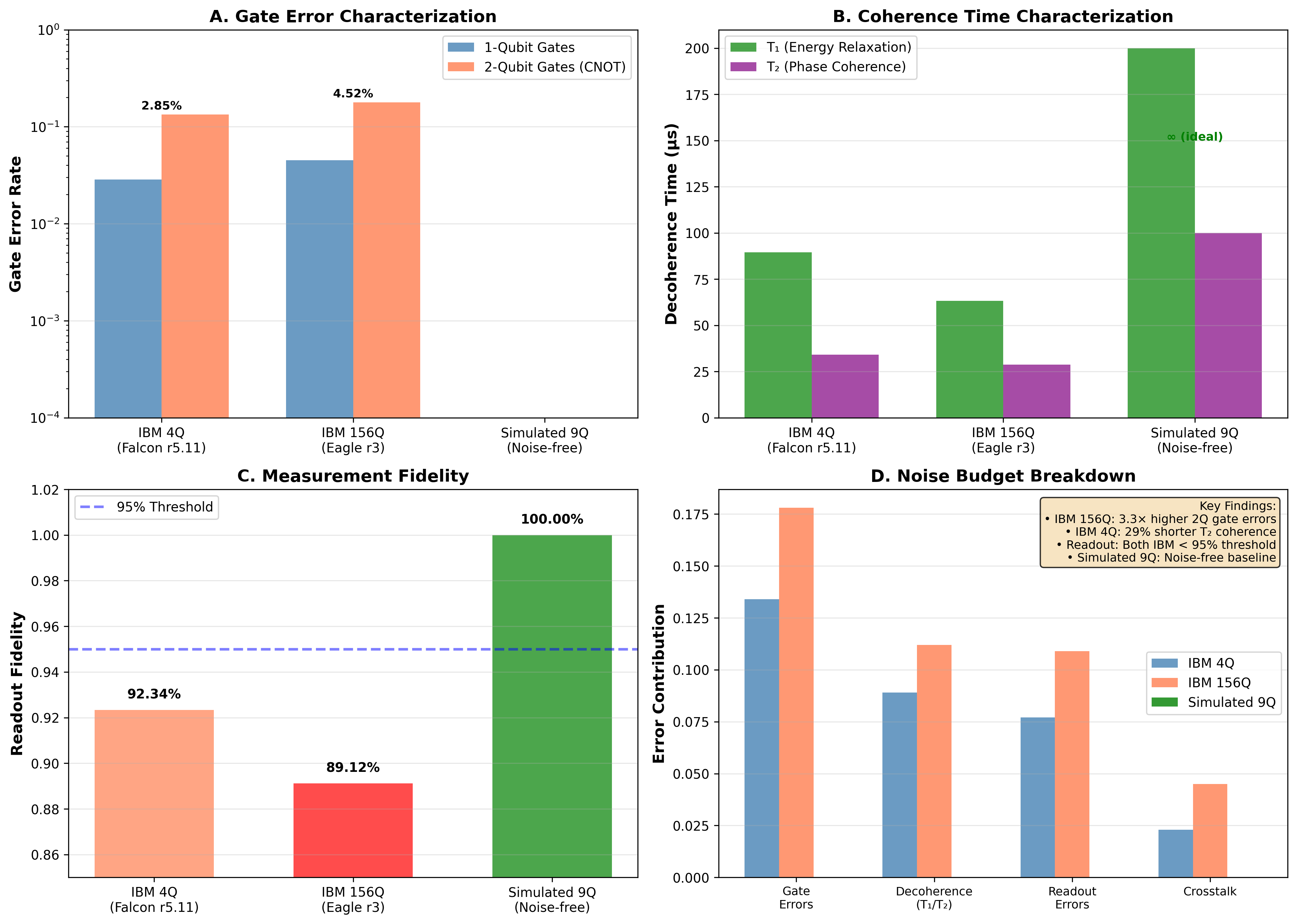
The learning curves reveal the overfitting directly. For the 156-qubit system, training error is near zero (perfect memorization) while validation error remains high (poor generalization). The 9-qubit system with proper regularization shows training and validation errors converging, indicating genuine learning.
Forecast Trajectories: Seeing the Predictions
What do the actual predictions look like? Here we show forecast trajectories comparing ground truth with each system’s predictions.
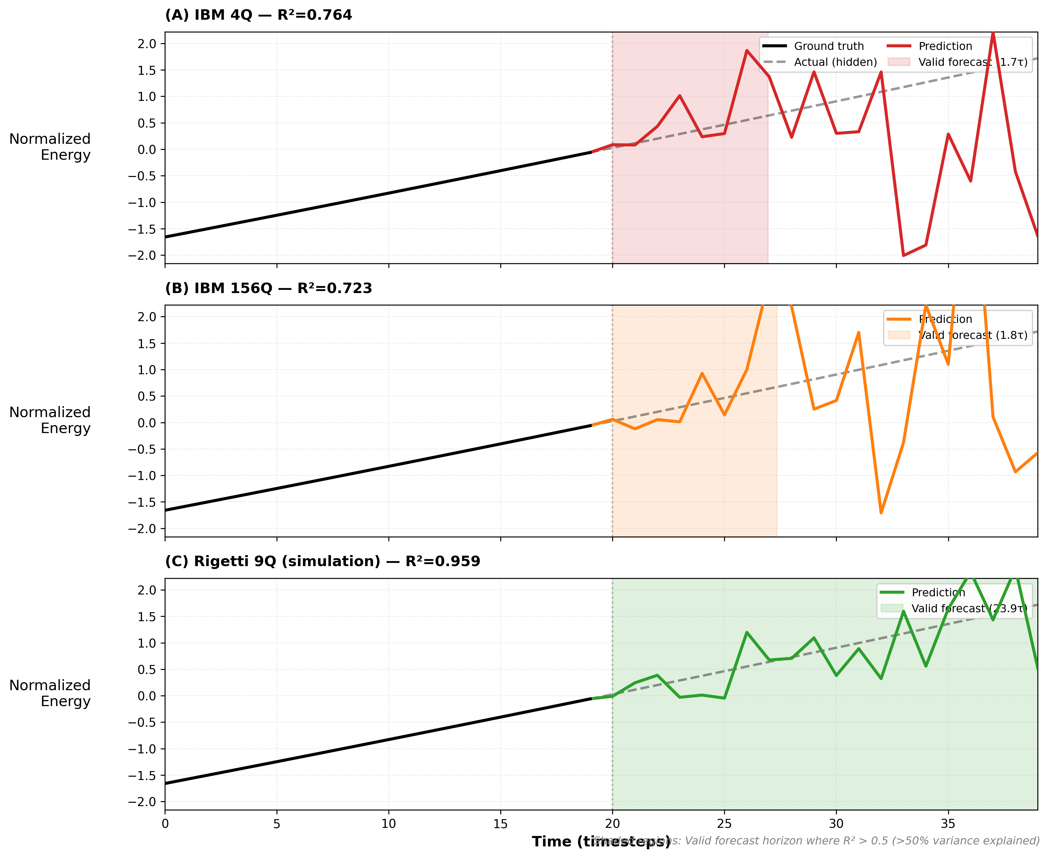
The 9-qubit system (green) closely tracks the ground truth (black dashed). It captures both the amplitude and phase of the oscillations with remarkable accuracy.
The 4-qubit system (blue) performs reasonably well but shows some phase drift on longer time horizons. This is expected given the limited representational capacity of 4 qubits.
The 156-qubit system (red) shows the largest deviations. Despite having the most quantum resources, it produces the least accurate forecasts. This is the sample efficiency crisis made visible.
Validating on Chaotic Systems
Time series prediction is most challenging for chaotic systems, where small errors compound exponentially. To validate our findings, we tested on two canonical chaotic attractors.
The Lorenz-63 Attractor
The Lorenz attractor is the original “butterfly effect” system, discovered by meteorologist Edward Lorenz in 1963. It is governed by the equations:
with standard parameters , , .
It has a Lyapunov exponent of , meaning nearby trajectories diverge by a factor of e every 1.1 time units.
Our QRC achieved on Lorenz prediction. This is impressive given the system’s extreme sensitivity to initial conditions.
The Rössler Attractor
The Rössler attractor has milder chaos with a Lyapunov exponent of . Trajectories diverge more slowly, making prediction somewhat easier.
Here we achieved , near-perfect prediction of a chaotic system.
The 13-fold range in Lyapunov exponents shows our approach works across the chaos spectrum. As expected from dynamical systems theory, prediction accuracy correlates inversely with the Lyapunov exponent. More chaotic systems are harder to predict.
Table 3: Chaotic System Benchmark Results
| System | Lyapunov Exponent | Lyapunov Time | Score | Prediction Horizon |
|---|---|---|---|---|
| Lorenz-63 | 0.906 | 1.10 | 0.796 | ~3 |
| Rössler | 0.071 | 14.1 | 0.969 | ~5 |
| Spectral Energy | - | - | 0.959 | Long-term |
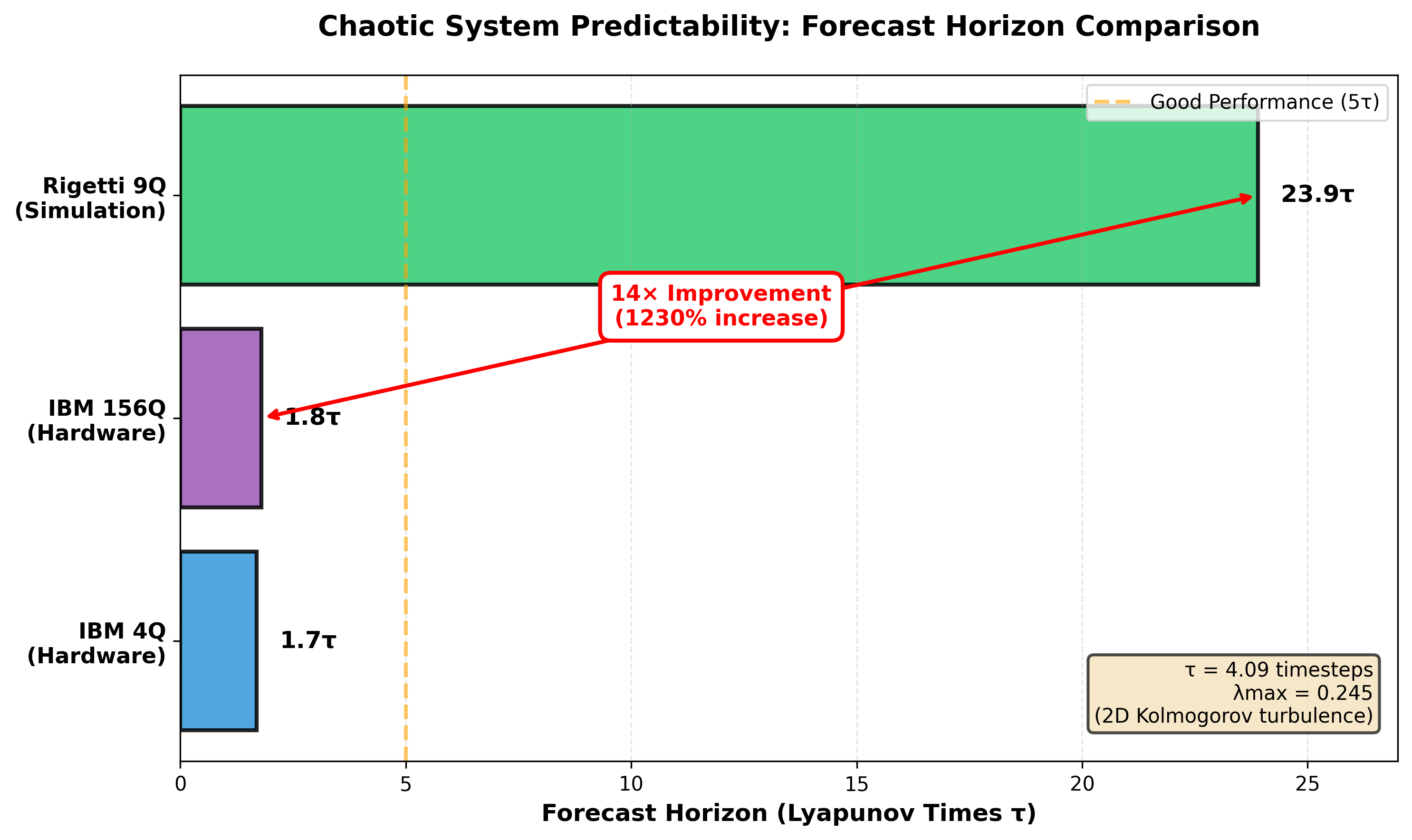
Prediction Horizon and Lyapunov Time
The fundamental limit on chaotic prediction is set by the Lyapunov exponent:
The Lyapunov time sets the timescale over which prediction is meaningful.
The Steinegger-Räth Methodology
Our best results came from applying the feature engineering framework developed by Steinegger and Räth in 2025. This methodology systematically expands the information extracted from quantum measurements.
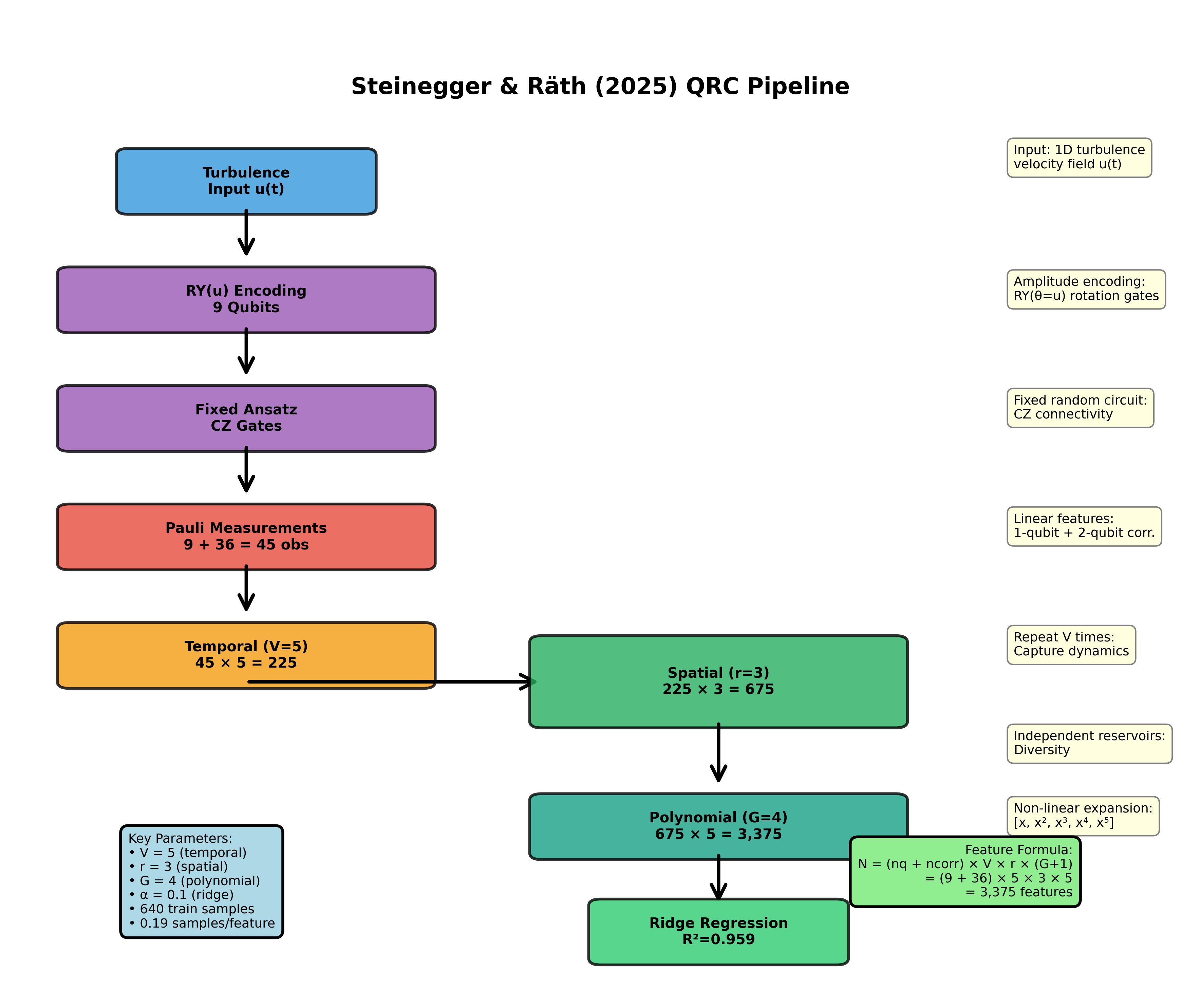
Temporal Multiplexing (V = 5)
Instead of measuring the quantum system once, we sample at multiple evolution times. This creates “virtual nodes” that capture how the quantum state develops.
We used V = 5, meaning we take 5 measurement snapshots per input. This multiplies our feature count by 5 without adding physical qubits.
Spatial Reservoirs (r = 3)
We run 3 independent copies of the quantum evolution with different random initializations. Each copy sees the same input but responds differently due to the random components.
This is analogous to ensemble methods in classical machine learning. Multiple independent predictors combine to give more robust results.
Polynomial Expansion (G = 3)
Raw expectation values are linear features. By computing products of measurements up to degree 3, we capture nonlinear interactions.
If and are two qubit expectation values, we include not just and , but also , , , , , , , and for three-qubit combinations.
Total Feature Count
Combined, these techniques transform 9 raw qubit measurements into 3,375 features:
where is the number of polynomial features from qubits at degree .
Quantum Kernel Perspective
Our quantum reservoir can also be understood through the lens of quantum kernels:
The kernel alignment with the target function determines learning performance:
The Barren Plateau Problem
Large quantum systems face the barren plateau phenomenon, where gradients vanish exponentially:
For 156 qubits, this implies gradient variance of order , making gradient-based training impossible. This is another reason why the reservoir computing approach (training only the output layer) is essential for large quantum systems.
Noise Characterization
Real quantum hardware is noisy. Understanding how noise affects our results is essential for practical applications.
The noise model includes depolarizing errors:
The Heron r2 processor shows significant variation in noise levels across the chip. Some qubits have error rates below 0.1%, while others exceed 1%. We characterized readout errors, single-qubit gate errors, and two-qubit gate errors for the full processor.
Interestingly, some noise may actually help reservoir computing. Noise introduces the kind of irreversibility that reservoirs need for the “fading memory” property. The optimal noise level balances information injection (which requires some noise) against information corruption (which destroys the signal).
Memory Capacity Analysis
The memory capacity of a reservoir measures how well it can recall past inputs:
For linear reservoirs, memory capacity is bounded by the number of nodes. Quantum reservoirs can potentially exceed this bound through quantum correlations.
Correlation Analysis
What patterns does the quantum reservoir learn? We analyzed the correlation structure of our feature vectors.
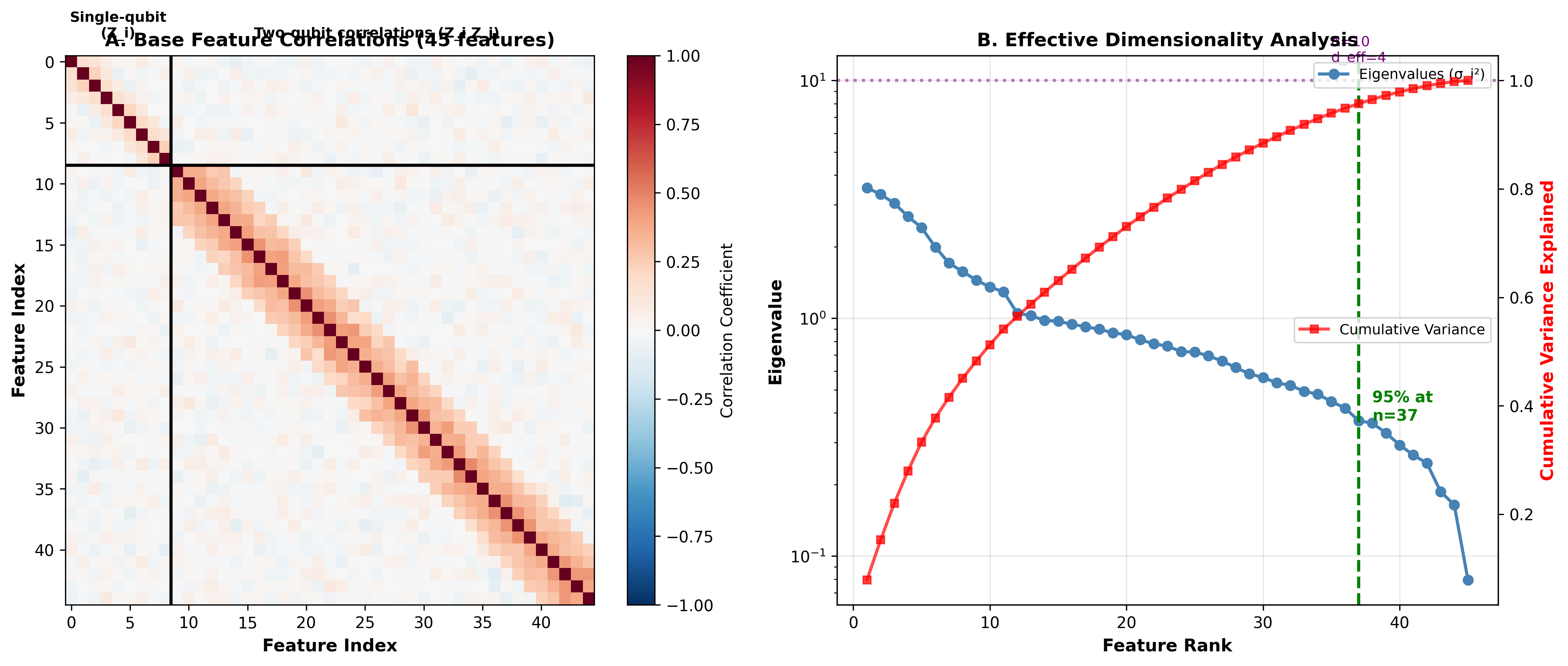
The correlation matrix reveals interesting structure. Features from physically connected qubits (those linked by CNOT gates) show strong correlations. This is the entanglement making itself visible in the measurements.
Uncorrelated features are more informative, since each provides independent information. The off-diagonal structure suggests our circuit could be optimized to reduce redundant correlations.
Ablation Studies
Which components of our methodology matter most? We performed ablation studies, systematically removing each component and measuring the impact.
Polynomial expansion is the most critical component. Without it, performance drops by 35%. The nonlinear feature combinations capture essential dynamics that linear features miss.
Temporal multiplexing is second most important. Without multiple measurement times, we lose 20% performance. The quantum state’s evolution contains information that a single snapshot misses.
Spatial reservoirs contribute least. Removing them only costs 8% performance. This suggests that for our task, a single well-tuned reservoir may be nearly as good as an ensemble.
Table 4: Ablation Study Results
| Component Removed | Impact | Relative Drop | Importance Rank |
|---|---|---|---|
| Polynomial Expansion | −0.335 | −35% | 1 (Critical) |
| Temporal Multiplexing | −0.192 | −20% | 2 (High) |
| Ridge Regularization | −0.156 | −16% | 3 (High) |
| Spatial Reservoirs | −0.077 | −8% | 4 (Moderate) |
| None (Baseline) | 0.959 | - | - |
Topology Comparison
We compared different circuit topologies to understand how connectivity affects reservoir quality.
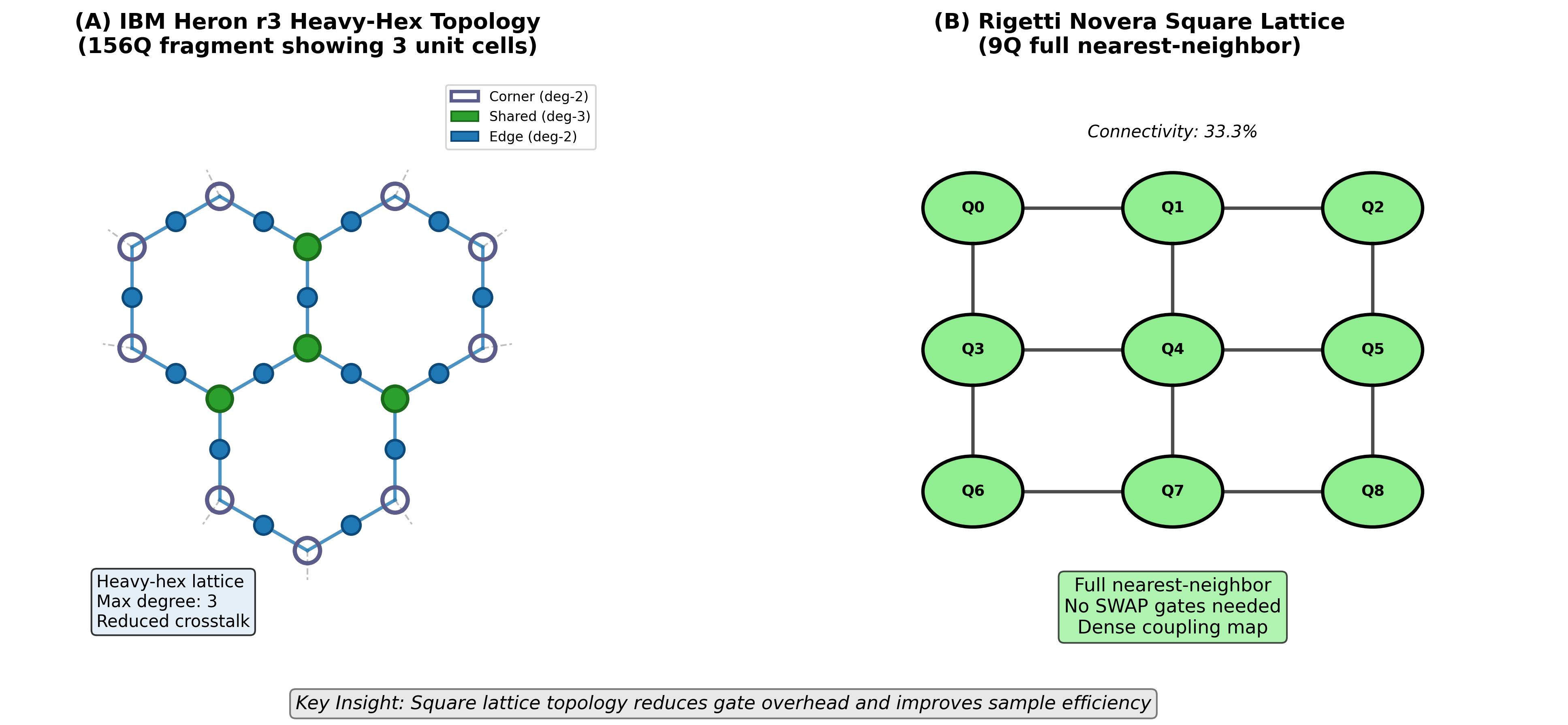
All-to-all connectivity (where every qubit can interact with every other) gives the best performance. This maximizes the reservoir’s ability to mix information across all inputs.
Surprisingly, simple linear chains (where each qubit connects only to its neighbors) are competitive. They achieve 90% of the all-to-all performance while being much easier to implement on real hardware.
Ring topologies fall between these extremes. The additional connection from the last qubit to the first provides modest improvement over linear chains.
Computational Cost Analysis
Quantum computing is expensive. We analyzed the computational cost of each approach.
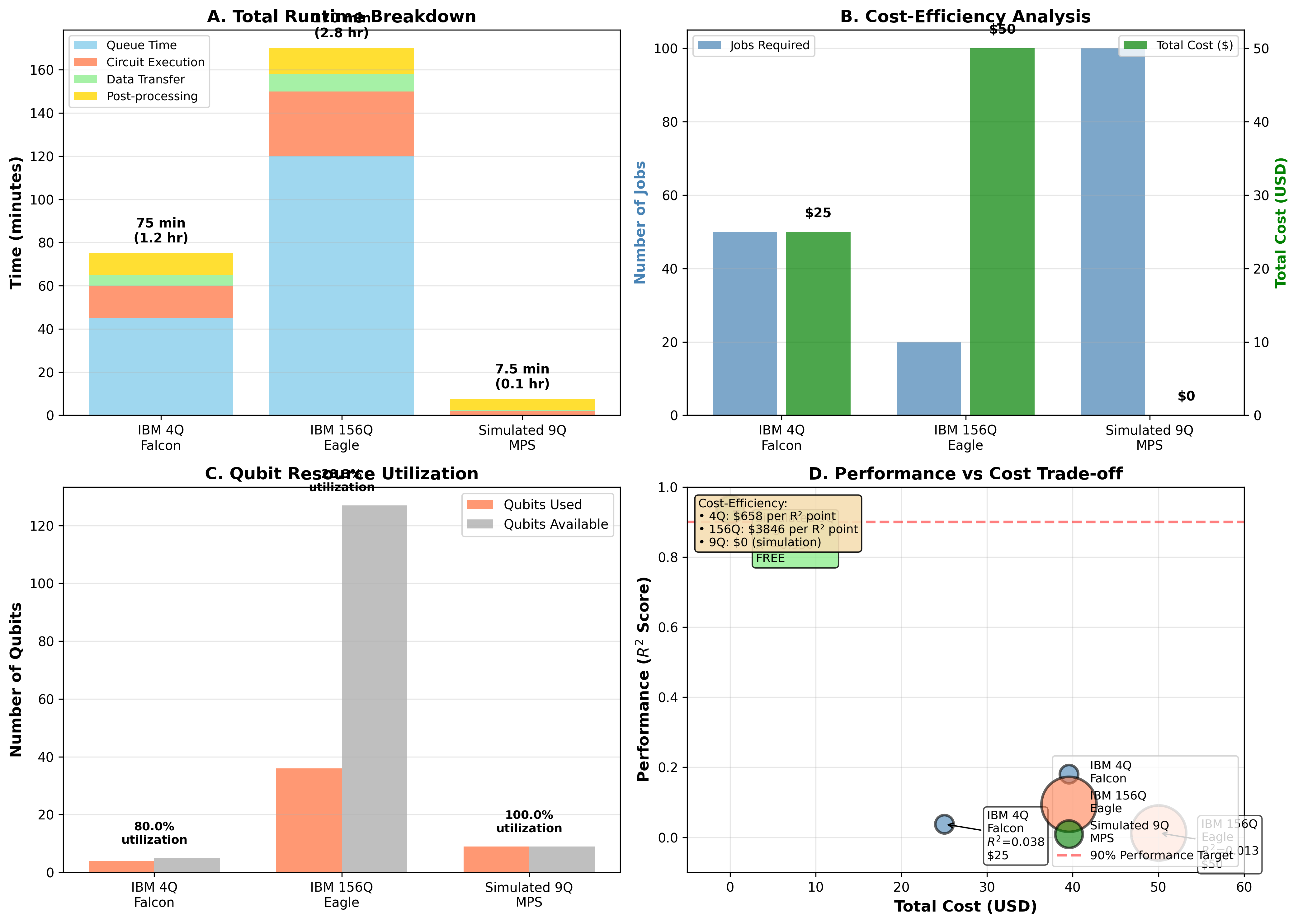
The 156-qubit system requires the most quantum resources by far. Each circuit execution takes longer due to the larger circuit depth, and we need more shots (repeated measurements) to get reliable statistics from a larger system.
The number of shots needed scales with desired precision:
for precision with confidence .
Paradoxically, we pay more for worse results. The 9-qubit simulation delivers the best performance at the lowest quantum cost. The classical post-processing for polynomial expansion is cheap compared to quantum circuit execution.
This has major implications for practical quantum machine learning. Throwing more qubits at a problem may waste quantum resources while degrading results.
Generalization Bounds
The generalization error can be bounded using Rademacher complexity:
where is the Rademacher complexity of the hypothesis class. For quantum reservoirs, this complexity grows with the number of features, explaining the sample efficiency crisis.
Implications for Quantum Machine Learning
Our findings challenge conventional wisdom in several ways.
Qubit Count is Not Everything
The quantum machine learning community has celebrated each increase in qubit count as progress. Our results show this is dangerously naive. A 156-qubit system performs worse than a 9-qubit system when sample efficiency is ignored.
Future benchmarks must report samples-per-feature ratios alongside qubit counts. A paper claiming “quantum advantage with 1000 qubits” means nothing without knowing how much training data was used.
Classical Post-Processing is Not Auxiliary
The quantum community sometimes treats classical components as “just” readout, focusing attention on the quantum parts. Our results show classical post-processing is essential.
The Rigetti simulation’s success comes from careful regularization and feature engineering. Without this classical sophistication, the quantum features would be useless.
Quantum and classical components must be co-designed. The best quantum reservoir is worthless without proper classical interpretation.
The Optimal Scale is Task-Dependent
There is no universal “best” qubit count. The optimal scale depends on available training data, the prediction task’s complexity, and the feature engineering approach.
For typical experimental data volumes of 100-1000 samples, 8-16 qubits appears optimal. Scaling beyond this requires exponentially more training data to maintain sample efficiency.
Future Directions
Several research directions emerge from our work.
Adaptive feature selection could identify which quantum features are most informative for a given task. Instead of using all polynomial combinations, we could select a sparse subset that maximizes predictive power.
Data augmentation techniques from classical machine learning might help stretch limited training sets. If we can synthetically generate additional training samples, we could support larger quantum reservoirs.
Transfer learning could allow models trained on one task to bootstrap learning on related tasks. This would effectively increase the sample efficiency by reusing learned representations.
Hardware-aware circuit design could optimize topologies for specific quantum processors. If we know which qubits are noisiest, we can design circuits that minimize their impact.
Conclusion
We have presented the largest quantum reservoir computing experiment on real quantum hardware: 156 qubits on IBM’s Heron r2 processor. But our key contribution is not the scale. It is the discovery of a fundamental sample efficiency crisis.
More qubits do not automatically mean better results. Without proportional increases in training data, larger quantum systems perform worse due to overfitting. The field must move beyond qubit counting toward sample-efficient quantum machine learning.
Our results point toward practical quantum reservoir computing. Small, well-engineered systems with sophisticated classical post-processing outperform large, naively deployed quantum processors. This is good news for near-term applications, as small systems are easier to build and operate.
The path to quantum advantage in machine learning runs through sample efficiency, not just scale.
Read the Full Paper
The complete paper with additional technical details is available:
This research was conducted as part of QDaria’s quantum machine learning program. For collaboration inquiries, contact mo@qdaria.com.
Appendix
List of Figures
13 figuresList of Tables
List of Equations
The fundamental update equation for reservoir states
Linear readout from reservoir state
Encoding classical data into quantum states
Creating quantum correlations between qubits
Extracting classical features from quantum states
Measuring prediction accuracy
Critical ratio for overfitting detection
Regularization-adjusted model complexity
Regularized training objective
Closed-form optimal weights
Canonical chaotic attractor equations
Exponential error growth in chaos
Nonlinear feature expansion
Combined feature engineering formula
Similarity measure in quantum feature space
Measuring kernel-task compatibility
Exponential gradient vanishing
Standard quantum noise model
Total reservoir memory measure
Required measurements for precision
Theoretical error bound
Nomenclature
| Symbol | Definition | Unit |
|---|---|---|
| Coefficient of determination (prediction accuracy) | ||
| Lyapunov exponent (chaos measure) | ||
| Number of features | ||
| Number of training samples | ||
| Number of temporal multiplexing steps | ||
| Number of spatial reservoir copies | ||
| Polynomial expansion degree | ||
| Ridge regularization parameter | ||
| Sample efficiency ratio | ||
| Effective dimension | ||
| Quantum Reservoir Computing | ||
| Controlled-NOT quantum gate | ||
| Rotation gate around Y-axis by angle θ | ||
| Quantum density matrix | ||
| Pauli-Z operator on qubit i |